Lean 4 定理证明
作者:Jeremy Avigad, Leonardo de Moura, Soonho Kong and Sebastian Ullrich, 以及Lean社区 译者 subfish_zhou
本中文教程旨在教你使用Lean 4。 参考Lean 4 Manual中的Setting Up Lean section一节来安装Lean。本项目也包括一个快速安装教程。 本书的Lean 2 和Lean 3 版本见这里。
本项目的翻译量较大,因此大多采用机翻,仅供习惯中文的读者作为参考,译者推荐有能力的读者阅读原文。欢迎对本译文提出宝贵意见,可邮件至subfishzhou@gmail.com 译者自制的习题参考答案在本项目Github仓库的Exercise文件夹中。本项目尚未完工。
介绍
计算机和定理证明
形式验证(Formal verification)是指使用逻辑和计算方法来验证用精确的数学术语表达的命题。这包括普通的数学定理,以及硬件或软件、网络协议、机械和混合系统中的形式命题。在实践中,验证数学命题和验证系统的正确性之间很类似:形式验证用数学术语描述硬件和软件系统,在此基础上验证其命题的正确性,这就像定理证明的过程。相反,一个数学定理的证明可能需要冗长的计算,在这种情况下,验证定理的真实性需要验证计算过程是否出错。
二十世纪的逻辑学发展表明,绝大多数传统证明方法可以化为若干基础系统中的一小套公理和规则。有了这种简化,计算机能以两种方式帮助建立命题:1)它可以帮助寻找一个证明,2)可以帮助验证一个所谓的证明是正确的。
自动定理证明(Automated theorem proving)着眼于 "寻找" 证明。归结(Resolution)定理证明器、表格法(tableau)定理证明器、快速可满足性求解器(fast satisfiability solvers)等提供了在命题逻辑和一阶逻辑中验证公式有效性的方法;还有些系统为特定的语言和问题提供搜索和决策程序,例如整数或实数上的线性或非线性表达式;像SMT(satisfiability modulo theories)这样的架构将通用的搜索方法与特定领域的程序相结合;计算机代数系统和专门的数学软件包提供了进行数学计算或寻找数学对象的手段,这些系统中的计算也可以被看作是一种证明,而这些系统也可以帮助建立数学命题。
自动推理系统努力追求能力和效率,但往往牺牲稳定性。这样的系统可能会有bug,而且很难保证它们所提供的结果是正确的。相比之下,交互式定理证明器侧重于 "验证" 证明,要求每个命题都有合适的公理基础的证明来支持。这就设定了非常高的标准:每一条推理规则和每一步计算都必须通过求助于先前的定义和定理来证明,一直到基本公理和规则。事实上,大多数这样的系统提供了精心设计的 "证明对象",可以传给其他系统并独立检查。构建这样的证明通常需要用户更多的输入和交互,但它可以让你获得更深入、更复杂的证明。
Lean 定理证明器旨在融合交互式和自动定理证明,它将自动化工具和方法置于一个支持用户交互和构建完整公理化证明的框架中。它的目标是支持数学推理和复杂系统的推理,并验证这两个领域的命题。
Lean的底层逻辑有一个计算的解释,与此同时Lean可以被视为一种编程语言。更重要的是,它可以被看作是一个编写具有精确语义的程序的系统,以及对程序所表示的计算功能进行推理。Lean中也有机制使它能够作为它自己的元编程语言,这意味着你可以使用Lean本身实现自动化和扩展Lean的功能。Lean的这些方面将在本教程的配套教程Lean 4编程中进行探讨,本书只介绍计算方面。
关于Lean
Lean 项目由微软雷德蒙德研究院的Leonardo de Moura在2013年发起,这是个长期项目,自动化方法的潜力会在未来逐步被挖掘。Lean是在Apache 2.0 license下发布的,这是一个允许他人自由使用和扩展代码和数学库的许可性开源许可证。
通常有两种办法来运行Lean。第一个是网页版本:由Javascript编写,包含标准定义和定理库,编辑器会下载到你的浏览器上运行。这是个方便快捷的办法。
第二种是本地版本:本地版本远快于网页版本,并且非常灵活。Visual Studio Code和Emacs扩展模块给编写和调试证明提供了有力支撑,因此更适合正式使用。源代码和安装方法见https://github.com/leanprover/lean4/.
本教程介绍的是Lean的当前版本:Lean 4。
关于本书
本书的目的是教你在Lean中编写和验证证明,并且不太需要针对Lean的基础知识。首先,你将学习Lean所基于的逻辑系统,它是依值类型论(dependent type theory)的一个版本,足以证明几乎所有传统的数学定理,并且有足够的表达能力自然地表示数学定理。更具体地说,Lean是基于具有归纳类型(inductive type)的构造演算(Calculus of Construction)系统的类型论版本。Lean不仅可以定义数学对象和表达依值类型论的数学断言,而且还可以作为一种语言来编写证明。
由于完全深入细节的公理证明十分复杂,定理证明的难点在于让计算机尽可能多地填补证明细节。你将通过依值类型论语言来学习各种方法实现自动证明,例如项重写,以及Lean中的项和表达式的自动简化方法。同样,繁饰(elaboration)和类型推理(type inference)的方法,可以用来支持灵活的代数推理。
最后,你会学到Lean的一些特性,包括与系统交流的语言,和Lean提供的对复杂理论和数据的管理机制。
在本书中你会见到类似下面这样的代码:
theorem and_commutative (p q : Prop) : p ∧ q → q ∧ p :=
  fun hpq : p ∧ q =>
  have hp : p := And.left hpq
  have hq : q := And.right hpq
  show q ∧ p from And.intro hq hp
你可以在Lean在线编辑器中尝试运行这些代码。(译者注:该编辑器速度很慢,且目前只支持Lean 3,但足够运行本书中大多数代码,仅需微小的语法改动。)
致谢
This tutorial is an open access project maintained on Github. Many people have contributed to the effort, providing corrections, suggestions, examples, and text. We are grateful to Ulrik Buchholz, Kevin Buzzard, Mario Carneiro, Nathan Carter, Eduardo Cavazos, Amine Chaieb, Joe Corneli, William DeMeo, Marcus Klaas de Vries, Ben Dyer, Gabriel Ebner, Anthony Hart, Simon Hudon, Sean Leather, Assia Mahboubi, Gihan Marasingha, Patrick Massot, Christopher John Mazey, Sebastian Ullrich, Floris van Doorn, Daniel Velleman, Théo Zimmerman, Paul Chisholm, and Chris Lovett for their contributions. Please see lean prover and lean community for an up to date list of our amazing contributors.
kokic、Faputa修改了n处typo,rujia liu审校了译本,toaster对改进译本提出了诸多宝贵建议,译者在此表示感谢。
安装Lean
(updates in 2023.09.17)
本教程演示在Windows系统下如何安装Lean 4正式版。Linux和MacOS版本请参考Lean Manual。
如果你身在中国,在运行安装程序前需要做如下准备:
在系统目录C:\Windows\System32\drivers\etc文件夹下找到hosts文件。对于其它系统用户也都是找到各自系统的hosts文件。
这个文件需要管理员权限来修改,有一个简便方法是,把它复制到别的地方修改,然后再粘贴回去,并选择使用管理员身份继续。
用记事本打开这个文件,在最后一行写入
185.199.108.133 raw.githubusercontent.com重启电脑,然后开启科学上网。(注意,你需要让终端也处在梯子的作用域中,例如你使用clash类梯子需要打开全局模式。)
(经过这个步骤之后你也可以使用官网提供的方法来安装了。)
如果你遇到"SSL connect error", "Timeout was reached","Failed to connect to github.com port 443"...等错误,就是说明你的网络环境有问题。重启电脑或者检查你的梯子。
基本安装
所有受支持平台的发布版本都可以在https://github.com/leanprover/lean4/releases中找到。
-
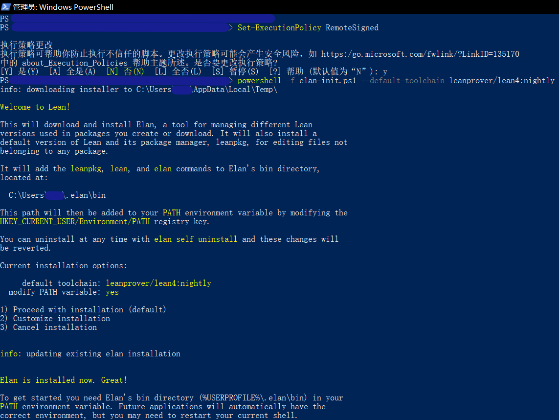
使用Lean版本管理器elan代替下载文件和手动设置路径。
在elan的Github仓库中下载最新release(对于windows,请下载elan-x86_64-pc-windows-msvc.zip),解压运行elan-init.exe,按照指示安装。
默认安装位置是用户文件目录下的
.elan文件夹,添加环境变量你的用户文件目录\.elan\bin。可能出现以下报错无法加载文件……因为在此系统上禁止运行此脚本”。解决方案是
1.用管理员身份运行Powershell;
2.输入命令
set-Executionpolicy Remotesigned,选择Y;然后就可以正常使用了。考虑到系统安全性,建议安装完成后将该选项改回默认值
N。效果如下图
由于本网站无法提供讨论区,欢迎向译者提供新的报错和解决方案,以丰富本页面。可邮件至subfishzhou@gmail.com
-
-
在终端中运行
$ elan self update # 以防你下载的不是最新版elan # 下载及应用最新的Lean4版本 (https://github.com/leanprover/lean4/releases) $ elan default leanprover/lean4:stable # 也可选择,只在当前目录下使用Lean4 $ elan override set leanprover/lean4:stable -
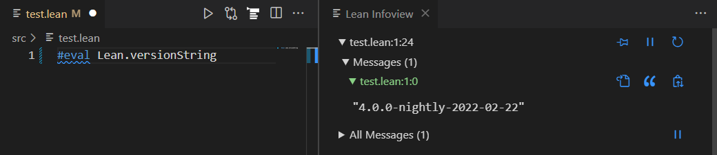
创建一个以
.lean为扩展名的新文件,并写入以下代码:#eval Lean.versionString你会看到语法高亮。当你把光标放在最后一行时,在右边有一个“Lean信息视图”,显示已经安装的Lean版本。
创建新Lean项目
用VS code打开一个新文件夹,你可以用两种方式创建新工程。
-
在终端中运行(
<your_project_name>替换为你自己起的名字)lake init <your_project_name>以创建一个名为your_project_name的空白新工程。如果你想把你的Lean程序编译成可执行文件,在终端中运行
lake build命令。如果你想在这个现有的工程中引用Mathlib4,你需要在
lakefile.lean文件中加入require mathlib from git "https://github.com/leanprover-community/mathlib4"然后在终端中运行
curl -L https://raw.githubusercontent.com/leanprover-community/mathlib4/master/lean-toolchain -o lean-toolchain -
如果你想直接创建一个引用Mathlib4的新工程,在终端中运行
lake +leanprover-community/mathlib4:lean-toolchain new <your_project_name> math以创建一个名为your_project_name的新工程。
使用Mathlib
更多内容请参考Mathlib Wiki
在你的项目文件夹下打开VS code,使用终端运行
lake update
lake exe cache get
如果你看到终端中显示了类似如下的提示:
Decompressing 1234 file(s)
unpacked in 12345 ms
同时你的项目文件夹中出现了lake-packages文件夹,那么证明你安装Mathlib成功了,重启系统即可使用。注意:你要在lake-packages所在的目录中运行VScode,才能让Lean使用Mathlib。
这里提供一个实例来测试你的安装:
import Mathlib.Data.Real.Basic
example (a b : ℝ) : a * b = b * a := by
  rw [mul_comm a b]
如果你的Lean infoview没有任何报错,并且光标放在文件最后一行时会提示“No goals”,证明你的Mathlib已经正确安装了。
如果你想更新Mathlib,在终端中运行
curl -L https://raw.githubusercontent.com/leanprover-community/mathlib4/master/lean-toolchain -o lean-toolchain
lake update
lake exe cache get
依值类型论
依值类型论(Dependent type theory)是一种强大而富有表达力的语言,允许你表达复杂的数学断言,编写复杂的硬件和软件规范,并以自然和统一的方式对这两者进行推理。Lean是基于一个被称为构造演算(Calculus of Constructions)的依值类型论的版本,它拥有一个可数的非累积性宇宙(non-cumulative universe)的层次结构以及归纳类型(inductive type)。在本章结束时,你将学会一大部分。
普通类型论
“类型论”得名于其中每个表达式都有一个类型。举例:在一个给定的语境中,x + 0可能表示一个自然数,f可能表示一个定义在自然数上的函数。Lean中的自然数是任意精度的无符号整数。
这里的一些例子展示了如何声明对象以及检查其类型。
/- 定义一些常数 -/

def m : Nat := 1       -- m 是自然数
def n : Nat := 0
def b1 : Bool := true  -- b1 是布尔型
def b2 : Bool := false

/- 检查类型 -/

#check m            -- 输出: Nat
#check n
#check n + 0        -- Nat
#check m * (n + 0)  -- Nat
#check b1           -- Bool
#check b1 && b2     -- "&&" is the Boolean and
#check b1 || b2     -- Boolean or
#check true         -- Boolean "true"

/- 求值(Evaluate) -/

#eval 5 * 4         -- 20
#eval m + 2         -- 3
#eval b1 && b2      -- false
位于/-和-/之间的文本组成了一个注释块,会被Lean的编译器忽略。类似地,两条横线--后面也是注释。注释块可以嵌套,这样就可以“注释掉”一整块代码,这和任何程序语言都是一样的。
def关键字声明工作环境中的新常量符号。在上面的例子中,def m : Nat := 1定义了一个Nat类型的新常量m,其值为1。#check命令要求Lean给出它的类型,用于向系统询问信息的辅助命令都以井号(#)开头。#eval命令让Lean计算给出的表达式。你应该试试自己声明一些常量和检查一些表达式的类型。
普通类型论的强大之处在于,你可以从其他类型中构建新的类型。例如,如果a和b是类型,a -> b表示从a到b的函数类型,a × b表示由a元素与b元素配对构成的类型,也称为笛卡尔积。注意×是一个Unicode符号,可以使用\times或简写\tim来输入。合理使用Unicode提高了易读性,所有现代编辑器都支持它。在Lean标准库中,你经常看到希腊字母表示类型,Unicode符号→是->的更紧凑版本。
#check Nat → Nat      -- 用"\to" or "\r"来打出这个箭头
#check Nat -> Nat     -- 也可以用 ASCII 符号

#check Nat × Nat      -- 用"\times"打出乘号
#check Prod Nat Nat   -- 换成ASCII 符号

#check Nat → Nat → Nat
#check Nat → (Nat → Nat)  --  结果和上一个一样

#check Nat × Nat → Nat
#check (Nat → Nat) → Nat -- 一个“泛函”

#check Nat.succ     -- Nat → Nat
#check (0, 1)       -- Nat × Nat
#check Nat.add      -- Nat → Nat → Nat

#check Nat.succ 2   -- Nat
#check Nat.add 3    -- Nat → Nat
#check Nat.add 5 2  -- Nat
#check (5, 9).1     -- Nat
#check (5, 9).2     -- Nat

#eval Nat.succ 2   -- 3
#eval Nat.add 5 2  -- 7
#eval (5, 9).1     -- 5
#eval (5, 9).2     -- 9
同样,你应该自己尝试一些例子。
让我们看一些基本语法。你可以通过输入\to或者\r或者\->来输入→。你也可以就用ASCII码->,所以表达式Nat -> Nat和Nat → Nat意思是一样的,都表示以一个自然数作为输入并返回一个自然数作为输出的函数类型。Unicode符号×是笛卡尔积,用\times输入。小写的希腊字母α,β,和γ等等常用来表示类型变量,可以用\a,\b,和\g来输入。
这里还有一些需要注意的事情。第一,函数f应用到值x上写为f x(例:Nat.succ 2)。第二,当写类型表达式时,箭头是右结合的;例如,Nat.add的类型是Nat → Nat → Nat,等价于Nat → (Nat → Nat)。
因此你可以把Nat.add看作一个函数,它接受一个自然数并返回另一个函数,该函数接受一个自然数并返回一个自然数。在类型论中,把Nat.add函数看作接受一对自然数作为输入并返回一个自然数作为输出的函数通常会更方便。系统允许你“部分应用”函数Nat.add,比如Nat.add 3具有类型Nat → Nat,即Nat.add 3返回一个“等待”第二个参数n的函数,然后可以继续写Nat.add 3 n。
注:取一个类型为
Nat × Nat → Nat的函数,然后“重定义”它,让它变成Nat → Nat → Nat类型,这个过程被称作柯里化(currying)。
如果你有m : Nat和n : Nat,那么(m, n)表示m和n组成的有序对,其类型为Nat × Nat。这个方法可以制造自然数对。反过来,如果你有p : Nat × Nat,之后你可以写p.1 : Nat和p.2 : Nat。这个方法用于提取它的两个组件。
类型作为对象
Lean所依据的依值类型论对普通类型论的其中一项升级是,类型本身(如Nat和Bool这些东西)也是对象,因此也具有类型。
#check Nat               -- Type
#check Bool              -- Type
#check Nat → Bool        -- Type
#check Nat × Bool        -- Type
#check Nat → Nat         -- ...
#check Nat × Nat → Nat
#check Nat → Nat → Nat
#check Nat → (Nat → Nat)
#check Nat → Nat → Bool
#check (Nat → Nat) → Nat
上面的每个表达式都是类型为Type的对象。你也可以为类型声明新的常量:
def α : Type := Nat
def β : Type := Bool
def F : Type → Type := List
def G : Type → Type → Type := Prod

#check α        -- Type
#check F α      -- Type
#check F Nat    -- Type
#check G α      -- Type → Type
#check G α β    -- Type
#check G α Nat  -- Type
正如上面所示,你已经看到了一个类型为Type → Type → Type的函数例子,即笛卡尔积 Prod:
def α : Type := Nat
def β : Type := Bool

#check Prod α β       -- Type
#check α × β          -- Type

#check Prod Nat Nat   -- Type
#check Nat × Nat      -- Type
这里有另一个例子:给出任意类型α,那么类型List α是类型为α的元素的列表的类型。
def α : Type := Nat

#check List α    -- Type
#check List Nat  -- Type
看起来Lean中任何表达式都有一个类型,因此你可能会想到:Type自己的类型是什么?
#check Type -- Type 1
实际上,这是Lean系统的一个最微妙的方面:Lean的底层基础有无限的类型层次:
#check Type     -- Type 1
#check Type 1   -- Type 2
#check Type 2   -- Type 3
#check Type 3   -- Type 4
#check Type 4   -- Type 5
可以将Type 0看作是一个由“小”或“普通”类型组成的宇宙。然后,Type 1是一个更大的类型范围,其中包含Type 0作为一个元素,而Type 2是一个更大的类型范围,其中包含Type 1作为一个元素。这个列表是不确定的,所以对于每个自然数n都有一个Type n。Type是Type 0的缩写:
#check Type
#check Type 0
然而,有些操作需要在类型宇宙上具有多态(polymorphic)。例如,List α应该对任何类型的α都有意义,无论α存在于哪种类型的宇宙中。所以函数List有如下的类型:
#check List -- Type u_1 → Type u_1
这里u_1是一个覆盖类型级别的变量。#check命令的输出意味着当α有类型Type n时,List α也有类型Type n。函数Prod具有类似的多态性:
#check Prod -- Type u_1 → Type u_2 → Type (max u_1 u_2)
你可以使用 universe 命令来声明宇宙变量,这样就可以定义多态常量:
universe u

def F (α : Type u) : Type u := Prod α α

#check F    -- Type u → Type u
可以通过在定义F时提供universe参数来避免使用universe命令:
def F.{u} (α : Type u) : Type u := Prod α α

#check F    -- Type u → Type u
函数抽象和求值
Lean提供 fun (或 λ)关键字用于从给定表达式创建函数,如下所示:
#check fun (x : Nat) => x + 5   -- Nat → Nat
#check λ (x : Nat) => x + 5     -- λ 和 fun 是同义词
#check fun x : Nat => x + 5     -- 同上
#check λ x : Nat => x + 5       -- 同上
你可以通过传递所需的参数来计算lambda函数:
#eval (λ x : Nat => x + 5) 10 -- 15
从另一个表达式创建函数的过程称为lambda 抽象。假设你有一个变量x : α和一个表达式t : β,那么表达式fun (x : α) => t或者λ (x : α) => t是一个类型为α → β的对象。这个从α到β的函数把任意x映射到t。
这有些例子:
#check fun x : Nat => fun y : Bool => if not y then x + 1 else x + 2
#check fun (x : Nat) (y : Bool) => if not y then x + 1 else x + 2
#check fun x y => if not y then x + 1 else x + 2   -- Nat → Bool → Nat
Lean将这三个例子解释为相同的表达式;在最后一个表达式中,Lean可以从表达式if not y then x + 1 else x + 2推断x和y的类型。
一些数学上常见的函数运算的例子可以用lambda抽象的项来描述:
def f (n : Nat) : String := toString n
def g (s : String) : Bool := s.length > 0

#check fun x : Nat => x        -- Nat → Nat
#check fun x : Nat => true     -- Nat → Bool
#check fun x : Nat => g (f x)  -- Nat → Bool
#check fun x => g (f x)        -- Nat → Bool
看看这些表达式的意思。表达式fun x : Nat => x代表Nat上的恒等函数,表达式fun x : Nat => true表示一个永远输出true的常值函数,表达式fun x : Nat => g (f x)表示f和g的复合。一般来说,你可以省略类型注释,让Lean自己推断它。因此你可以写fun x => g (f x)来代替fun x : Nat => g (f x)。
你可以以函数作为参数,通过给它们命名f和g,你可以在实现中使用这些函数:
#check fun (g : String → Bool) (f : Nat → String) (x : Nat) => g (f x)
-- (String → Bool) → (Nat → String) → Nat → Bool
你还可以以类型作为参数:
#check fun (α β γ : Type) (g : β → γ) (f : α → β) (x : α) => g (f x)
这个表达式表示一个接受三个类型α,β和γ和两个函数g : β → γ和f : α → β,并返回的g和f的复合的函数。(理解这个函数的类型需要理解依值乘积类型,下面将对此进行解释。)
lambda表达式的一般形式是fun x : α => t,其中变量x是一个“约束变量”:它实际上是一个占位符,其“作用域”没有扩展到表达式t之外。例如,表达式fun (b : β) (x : α) => b中的变量b与前面声明的常量b没有任何关系。事实上,这个表达式表示的函数与fun (u : β) (z : α) => u是一样的。形式上,可以通过给约束变量重命名来使形式相同的表达式被看作是alpha等价的,也就是被认为是“一样的”。Lean认识这种等价性。
注意到项t : α → β应用到项s : α上导出了表达式t s : β。回到前面的例子,为清晰起见给约束变量重命名,注意以下表达式的类型:
#check (fun x : Nat => x) 1     -- Nat
#check (fun x : Nat => true) 1  -- Bool

def f (n : Nat) : String := toString n
def g (s : String) : Bool := s.length > 0

#check
  (fun (α β γ : Type) (u : β → γ) (v : α → β) (x : α) => u (v x)) Nat String Bool g f 0
  -- Bool
表达式(fun x : Nat => x) 1的类型是Nat。实际上,应用(fun x : Nat => x)到1上返回的值是1。
#eval (fun x : Nat => x) 1     -- 1
#eval (fun x : Nat => true) 1  -- true
稍后你将看到这些项是如何计算的。现在,请注意这是依值类型论的一个重要特征:每个项都有一个计算行为,并支持“标准化”的概念。从原则上讲,两个可以化约为相同形式的项被称为“定义等价”。它们被Lean的类型检查器认为是“相同的”,并且Lean尽其所能地识别和支持这些识别结果。
Lean是个完备的编程语言。它有一个生成二进制可执行文件的编译器,和一个交互式解释器。你可以用#eval命令执行表达式,这也是测试你的函数的好办法。
注意到
#eval和#reduce不是等价的。#eval命令首先把Lean表达式编译成中间表示(intermediate representation, IR)然后用一个解释器来执行这个IR。某些内建类型(例如,Nat、String、Array)在IR中有更有效率的表示。IR支持使用对Lean不透明的外部函数。#reduce命令建立在一个化简引擎上,类似于在Lean的可信内核中使用的那个,它是负责检查和验证表达式和证明正确性的那一部分。它的效率不如#eval,且将所有外部函数视为不透明的常量。之后你将了解到这两个命令之间还有其他一些差异。
定义
def关键字提供了一个声明新对象的重要方式。
def double (x : Nat) : Nat :=
  x + x
这很类似其他编程语言中的函数。名字double被定义为一个函数,它接受一个类型为Nat的输入参数x,其结果是x + x,因此它返回类型Nat。然后你可以调用这个函数:
#eval double 3 -- 6
在这种情况下你可以把def想成一种lambda。下面给出了相同的结果:
def double :=
  fun (x : Nat) => x + x
当Lean有足够的信息来推断时,你可以省略类型声明。类型推断是Lean的重要组成部分:
def double : Nat → Nat :=
  fun x => x + x

#eval double 3    -- 6
定义的一般形式是def foo : α := bar,其中α是表达式bar返回的类型。Lean通常可以推断类型α,但是精确写出它可以澄清你的意图,并且如果定义的右侧没有匹配你的类型,Lean将标记一个错误。
bar可以是任何一个表达式,不只是一个lambda表达式。因此def也可以用于给一些值命名,例如:
def pi := 3.141592654
def可以接受多个输入参数。比如定义两自然数之和:
def add (x y : Nat) :=
  x + y

#eval add 3 2               -- 5
参数列表可以像这样分开写:
def add (x : Nat) (y : Nat) :=
  x + y

#eval add (double 3) (7 + 9)  -- 22
注意到这里我们使用了double函数来创建add函数的第一个参数。
你还可以在def中写一些更有趣的表达式:
def greater (x y : Nat) :=
  if x > y then x
  else y
你可能能猜到这个可以做什么。
还可以定义一个函数,该函数接受另一个函数作为输入。下面调用一个给定函数两次,将第一次调用的输出传递给第二次:
def doTwice (f : Nat → Nat) (x : Nat) : Nat :=
  f (f x)

#eval doTwice double 2   -- 8
现在为了更抽象一点,你也可以指定类型参数等:
def compose (α β γ : Type) (g : β → γ) (f : α → β) (x : α) : γ :=
  g (f x)
这句代码的意思是:函数compose首先接受任何两个函数作为参数,这其中两个函数各自接受一个输入。类型β → γ和α → β意思是要求第二个函数的输出类型必须与第一个函数的输入类型匹配,否则这两个函数将无法复合。
compose再接受一个类型为α的参数作为第二个函数(这里叫做f)的输入,通过这个函数之后的返回结果类型为β,再作为第一个函数(这里叫做g)的输入。第一个函数返回类型为γ,这就是compose函数最终返回的类型。
compose可以在任意的类型α β γ上使用,它可以复合任意两个函数,只要前一个的输出类型是后一个的输入类型。举例:
-- def compose (α β γ : Type) (g : β → γ) (f : α → β) (x : α) : γ :=
--  g (f x)
-- def double (x : Nat) : Nat :=
--  x + x
def square (x : Nat) : Nat :=
  x * x

#eval compose Nat Nat Nat double square 3  -- 18
局部定义
Lean还允许你使用let关键字来引入“局部定义”。表达式let a := t1; t2定义等价于把t2中所有的a替换成t1的结果。
#check let y := 2 + 2; y * y   -- Nat
#eval  let y := 2 + 2; y * y   -- 16

def twice_double (x : Nat) : Nat :=
  let y := x + x; y * y

#eval twice_double 2   -- 16
这里twice_double x定义等价于(x + x) * (x + x)。
你可以连续使用多个let命令来进行多次替换:
#check let y := 2 + 2; let z := y + y; z * z   -- Nat
#eval  let y := 2 + 2; let z := y + y; z * z   -- 64
换行可以省略分号;。
def t (x : Nat) : Nat :=
  let y := x + x
  y * y
表达式let a := t1; t2的意思很类似(fun a => t2) t1,但是这两者并不一样。前者中你要把t2中每一个a的实例考虑成t1的一个缩写。后者中a是一个变量,表达式fun a => t2不依赖于a的取值而可以单独具有意义。作为一个对照,考虑为什么下面的foo定义是合法的,但bar不行(因为在确定了x所属的a是什么之前,是无法让它+ 2的)。
def foo := let a := Nat; fun x : a => x + 2
/-
  def bar := (fun a => fun x : a => x + 2) Nat
-/
变量和小节
考虑下面这三个函数定义:
def compose (α β γ : Type) (g : β → γ) (f : α → β) (x : α) : γ :=
  g (f x)

def doTwice (α : Type) (h : α → α) (x : α) : α :=
  h (h x)

def doThrice (α : Type) (h : α → α) (x : α) : α :=
  h (h (h x))
Lean提供variable指令来让这些声明变得紧凑:
variable (α β γ : Type)

def compose (g : β → γ) (f : α → β) (x : α) : γ :=
  g (f x)

def doTwice (h : α → α) (x : α) : α :=
  h (h x)

def doThrice (h : α → α) (x : α) : α :=
  h (h (h x))
你可以声明任意类型的变量,不只是Type类型:
variable (α β γ : Type)
variable (g : β → γ) (f : α → β) (h : α → α)
variable (x : α)

def compose := g (f x)
def doTwice := h (h x)
def doThrice := h (h (h x))

#print compose
#print doTwice
#print doThrice
输出结果表明所有三组定义具有完全相同的效果。
variable命令指示Lean将声明的变量作为约束变量插入定义中,这些定义通过名称引用它们。Lean足够聪明,它能找出定义中显式或隐式使用哪些变量。因此在写定义时,你可以将α、β、γ、g、f、h和x视为固定的对象,并让Lean自动抽象这些定义。
当以这种方式声明时,变量将一直保持存在,直到所处理的文件结束。然而,有时需要限制变量的作用范围。Lean提供了小节标记section来实现这个目的:
section useful
  variable (α β γ : Type)
  variable (g : β → γ) (f : α → β) (h : α → α)
  variable (x : α)

  def compose := g (f x)
  def doTwice := h (h x)
  def doThrice := h (h (h x))
end useful
当一个小节结束后,变量不再发挥作用。
你不需要缩进一个小节中的行。你也不需要命名一个小节,也就是说,你可以使用一个匿名的section /end对。但是,如果你确实命名了一个小节,你必须使用相同的名字关闭它。小节也可以嵌套,这允许你逐步增加声明新变量。
命名空间
Lean可以让你把定义放进一个“命名空间”(namespace)里,并且命名空间也是层次化的:
namespace Foo
  def a : Nat := 5
  def f (x : Nat) : Nat := x + 7

  def fa : Nat := f a
  def ffa : Nat := f (f a)

  #check a
  #check f
  #check fa
  #check ffa
  #check Foo.fa
end Foo

-- #check a  -- error
-- #check f  -- error
#check Foo.a
#check Foo.f
#check Foo.fa
#check Foo.ffa

open Foo

#check a
#check f
#check fa
#check Foo.fa
当你声明你在命名空间Foo中工作时,你声明的每个标识符都有一个前缀Foo.。在打开的命名空间中,可以通过较短的名称引用标识符,但是关闭命名空间后,必须使用较长的名称。与section不同,命名空间需要一个名称。只有一个匿名命名空间在根级别上。
open命令使你可以在当前使用较短的名称。通常,当你导入一个模块时,你会想打开它包含的一个或多个命名空间,以访问短标识符。但是,有时你希望将这些信息保留在一个完全限定的名称中,例如,当它们与你想要使用的另一个命名空间中的标识符冲突时。因此,命名空间为你提供了一种在工作环境中管理名称的方法。
例如,Lean把和列表相关的定义和定理都放在了命名空间List之中。
#check List.nil
#check List.cons
#check List.map
open List命令允许你使用短一点的名字:
open List

#check nil
#check cons
#check map
像小节一样,命名空间也是可以嵌套的:
namespace Foo
  def a : Nat := 5
  def f (x : Nat) : Nat := x + 7

  def fa : Nat := f a

  namespace Bar
    def ffa : Nat := f (f a)

    #check fa
    #check ffa
  end Bar

  #check fa
  #check Bar.ffa
end Foo

#check Foo.fa
#check Foo.Bar.ffa

open Foo

#check fa
#check Bar.ffa
关闭的命名空间可以之后重新打开,甚至是在另一个文件里:
namespace Foo
  def a : Nat := 5
  def f (x : Nat) : Nat := x + 7

  def fa : Nat := f a
end Foo

#check Foo.a
#check Foo.f

namespace Foo
  def ffa : Nat := f (f a)
end Foo
与小节一样,嵌套的名称空间必须按照打开的顺序关闭。命名空间和小节有不同的用途:命名空间组织数据,小节声明变量,以便在定义中插入。小节对于分隔set_option和open等命令的范围也很有用。
然而,在许多方面,namespace ... end结构块和section ... end表现出来的特征是一样的。尤其是你在命名空间中使用variable命令时,它的作用范围被限制在命名空间里。类似地,如果你在命名空间中使用open命令,它的效果在命名空间关闭后消失。
依值类型论“依赖”着什么?
简单地说,类型可以依赖于参数。你已经看到了一个很好的例子:类型List α依赖于参数α,而这种依赖性是区分List Nat和List Bool的关键。另一个例子,考虑类型Vector α n,即长度为n的α元素的向量类型。这个类型取决于两个参数:向量中元素的类型α : Type和向量的长度n : Nat。
假设你希望编写一个函数cons,它在列表的开头插入一个新元素。cons应该有什么类型?这样的函数是多态的(polymorphic):你期望Nat,Bool或任意类型α的cons函数表现相同的方式。因此,将类型作为cons的第一个参数是有意义的,因此对于任何类型α,cons α是类型α列表的插入函数。换句话说,对于每个α,cons α是将元素a : α插入列表as : List α的函数,并返回一个新的列表,因此有cons α a as : List α。
很明显,cons α具有类型α → List α → List α,但是cons具有什么类型?如果我们假设是Type → α → list α → list α,那么问题在于,这个类型表达式没有意义:α没有任何的所指,但它实际上指的是某个类型Type。换句话说,假设α : Type是函数的首个参数,之后的两个参数的类型是α和List α,它们依赖于首个参数α。
def cons (α : Type) (a : α) (as : List α) : List α :=
  List.cons a as

#check cons Nat        -- Nat → List Nat → List Nat
#check cons Bool       -- Bool → List Bool → List Bool
#check cons            -- (α : Type) → α → List α → List α
这就是依值函数类型,或者依值箭头类型的一个例子。给定α : Type和β : α → Type,把β考虑成α之上的类型族,也就是说,对于每个a : α都有类型β a。在这种情况下,类型(a : α) → β a表示的是具有如下性质的函数f的类型:对于每个a : α,f a是β a的一个元素。换句话说,f返回值的类型取决于其输入。
注意到(a : α) → β对于任意表达式β : Type都有意义。当β的值依赖于a(例如,在前一段的表达式β a),(a : α) → β表示一个依值函数类型。当β的值不依赖于a,(a : α) → β与类型α → β无异。实际上,在依值类型论(以及Lean)中,α → β表达的意思就是当β的值不依赖于a时的(a : α) → β。【注】
译者注:在依值类型论的数学符号体系中,依值类型是用
Π符号来表达的,在Lean 3中还使用这种表达,例如Π x : α, β x。Lean 4抛弃了这种对新手不友好的写法,但是沿袭了三代中另外两种意义更明朗的写法:forall x : α, β x和∀ x : α, β x。这几个表达式都和(x : α) → β x同义。但是个人感觉本教程这一段的讲法也对新手不友好,(x : α) → β x这种写法在引入“构造子”之后意义会更明朗一些(见下一个注释),当前反倒是forall x : α, β x这种写法对于来自数学背景的读者更加清楚明白,关于前一种符号在量词与等价一章中有更详细的说明。同时,依值类型有着更丰富的引入动机,推荐读者寻找一些拓展读物。
回到列表的例子,你可以使用#check命令来检查下列的List函数。@符号以及圆括号和花括号之间的区别将在后面解释。
#check @List.cons    -- {α : Type u_1} → α → List α → List α
#check @List.nil     -- {α : Type u_1} → List α
#check @List.length  -- {α : Type u_1} → List α → Nat
#check @List.append  -- {α : Type u_1} → List α → List α → List α
就像依值函数类型(a : α) → β a通过允许β依赖α从而推广了函数类型α → β,依值笛卡尔积类型(a : α) × β a同样推广了笛卡尔积α × β。依值积类型又称为sigma类型,可写成Σ a : α, β a。你可以用⟨a, b⟩或者Sigma.mk a b来创建依值对。
universe u v

def f (α : Type u) (β : α → Type v) (a : α) (b : β a) : (a : α) × β a :=
  ⟨a, b⟩

def g (α : Type u) (β : α → Type v) (a : α) (b : β a) : Σ a : α, β a :=
  Sigma.mk a b

def h1 (x : Nat) : Nat :=
  (f Type (fun α => α) Nat x).2

#eval h1 5 -- 5

def h2 (x : Nat) : Nat :=
  (g Type (fun α => α) Nat x).2

#eval h2 5 -- 5
函数f和g表达的是同样的函数。
隐参数
假设我们有一个列表的实现如下:
universe u
def Lst (α : Type u) : Type u := List α
def Lst.cons (α : Type u) (a : α) (as : Lst α) : Lst α := List.cons a as
def Lst.nil (α : Type u) : Lst α := List.nil
def Lst.append (α : Type u) (as bs : Lst α) : Lst α := List.append as bs
#check Lst          -- Type u_1 → Type u_1
#check Lst.cons     -- (α : Type u_1) → α → Lst α → Lst α
#check Lst.nil      -- (α : Type u_1) → Lst α
#check Lst.append   -- (α : Type u_1) → Lst α → Lst α → Lst α
然后,你可以建立一个自然数列表如下:
#check Lst.cons Nat 0 (Lst.nil Nat)

def as : Lst Nat := Lst.nil Nat
def bs : Lst Nat := Lst.cons Nat 5 (Lst.nil Nat)

#check Lst.append Nat as bs
由于构造子对类型是多态的【注】,我们需要重复插入类型Nat作为一个参数。但是这个信息是多余的:我们可以推断表达式Lst.cons Nat 5 (Lst.nil Nat)中参数α的类型,这是通过第二个参数5的类型是Nat来实现的。类似地,我们可以推断Lst.nil Nat中参数的类型,这是通过它作为函数Lst.cons的一个参数,且这个函数在这个位置需要接收的是一个具有Lst α类型的参数来实现的。
译者注:“构造子”(constructor)的概念前文未加解释,对类型论不熟悉的读者可能会困惑。它指的是一种“依值类型的类型”,也可以看作“类型的构造器”,例如
λ α : α -> α甚至可看成⋆ -> ⋆。当给α或者⋆赋予一个具体的类型时,这个表达式就成为了一个类型。前文中(x : α) → β x中的β就可以看成一个构造子,(x : α)就是传进的类型参数。原句“构造子对类型是多态的”意为给构造子中放入不同类型时它会变成不同类型。
这是依值类型论的一个主要特征:项包含大量信息,而且通常可以从上下文推断出一些信息。在Lean中,我们使用下划线_来指定系统应该自动填写信息。这就是所谓的“隐参数”。
#check Lst.cons _ 0 (Lst.nil _)

def as : Lst Nat := Lst.nil _
def bs : Lst Nat := Lst.cons _ 5 (Lst.nil _)

#check Lst.append _ as bs
然而,敲这么多下划线仍然很无聊。当一个函数接受一个通常可以从上下文推断出来的参数时,Lean允许你指定该参数在默认情况下应该保持隐式。这是通过将参数放入花括号来实现的,如下所示:
universe u
def Lst (α : Type u) : Type u := List α

def Lst.cons {α : Type u} (a : α) (as : Lst α) : Lst α := List.cons a as
def Lst.nil {α : Type u} : Lst α := List.nil
def Lst.append {α : Type u} (as bs : Lst α) : Lst α := List.append as bs

#check Lst.cons 0 Lst.nil

def as : Lst Nat := Lst.nil
def bs : Lst Nat := Lst.cons 5 Lst.nil

#check Lst.append as bs
唯一改变的是变量声明中α : Type u周围的花括号。我们也可以在函数定义中使用这个技巧:
universe u
def ident {α : Type u} (x : α) := x

#check ident         -- ?m → ?m
#check ident 1       -- Nat
#check ident "hello" -- String
#check @ident        -- {α : Type u_1} → α → α
这使得ident的第一个参数是隐式的。从符号上讲,这隐藏了类型的说明,使它看起来好像ident只是接受任何类型的参数。事实上,函数id在标准库中就是以这种方式定义的。我们在这里选择一个非传统的名字只是为了避免名字的冲突。
variable命令也可以用这种技巧来来把变量变成隐式的:
universe u

section
  variable {α : Type u}
  variable (x : α)
  def ident := x
end

#check ident
#check ident 4
#check ident "hello"
Lean有非常复杂的机制来实例化隐参数,我们将看到它们可以用来推断函数类型、谓词,甚至证明。实例化这些“洞”或“占位符”的过程通常被称为繁饰(elaboration)。隐参数的存在意味着有时可能没有足够的信息来精确地确定表达式的含义。像id或List.nil这样的表达式被认为是“多态的”,因为它可以在不同的上下文中具有不同的含义。
可以通过写(e : T)来指定表达式e的类型T。这就指导Lean的繁饰器在试图解决隐式参数时使用值T作为e的类型。在下面的第二个例子中,这种机制用于指定表达式id和List.nil所需的类型:
#check List.nil               -- List ?m
#check id                     -- ?m → ?m

#check (List.nil : List Nat)  -- List Nat
#check (id : Nat → Nat)       -- Nat → Nat
Lean中数字是重载的,但是当数字的类型不能被推断时,Lean默认假设它是一个自然数。因此,下面的前两个#check命令中的表达式以同样的方式进行了繁饰,而第三个#check命令将2解释为整数。
#check 2            -- Nat
#check (2 : Nat)    -- Nat
#check (2 : Int)    -- Int
然而,有时我们可能会发现自己处于这样一种情况:我们已经声明了函数的参数是隐式的,但现在想显式地提供参数。如果foo是有隐参数的函数,符号@foo表示所有参数都是显式的该函数。
#check @id        -- {α : Type u_1} → α → α
#check @id Nat    -- Nat → Nat
#check @id Bool   -- Bool → Bool

#check @id Nat 1     -- Nat
#check @id Bool true -- Bool
第一个#check命令给出了标识符的类型id,没有插入任何占位符。而且,输出表明第一个参数是隐式的。
命题和证明
前一章你已经看到了在Lean中定义对象和函数的一些方法。在本章中,我们还将开始解释如何用依值类型论的语言来编写数学命题和证明。
命题即类型
证明在依值类型论语言中定义的对象的断言(assertion)的一种策略是在定义语言之上分层断言语言和证明语言。但是,没有理由以这种方式重复使用多种语言:依值类型论是灵活和富有表现力的,我们也没有理由不能在同一个总框架中表示断言和证明。
例如,我们可引入一种新类型Prop,来表示命题,然后引入用其他命题构造新命题的构造子。
def Implies (p q : Prop) : Prop := p → q
#check And     -- Prop → Prop → Prop
#check Or      -- Prop → Prop → Prop
#check Not     -- Prop → Prop
#check Implies -- Prop → Prop → Prop

variable (p q r : Prop)
#check And p q                      -- Prop
#check Or (And p q) r               -- Prop
#check Implies (And p q) (And q p)  -- Prop
对每个元素p : Prop,可以引入另一个类型Proof p,作为p的证明的类型。“公理”是这个类型中的常值。
structure Proof (p : Prop) : Type where
  proof : p
#check Proof   -- Proof : Prop → Type

axiom and_comm (p q : Prop) : Proof (Implies (And p q) (And q p))

variable (p q : Prop)
#check and_comm p q     -- Proof (Implies (And p q) (And q p))
然而,除了公理之外,我们还需要从旧证明中建立新证明的规则。例如,在许多命题逻辑的证明系统中,我们有肯定前件式(modus ponens)推理规则:
如果能证明
Implies p q和p,则能证明q。
我们可以如下地表示它:
axiom modus_ponens : (p q : Prop) → Proof (Implies p q) → Proof p → Proof q
命题逻辑的自然演绎系统通常也依赖于以下规则:
当假设
p成立时,如果我们能证明q. 则我们能证明Implies p q.
我们可以如下地表示它:
axiom implies_intro : (p q : Prop) → (Proof p → Proof q) → Proof (Implies p q)
这个功能让我们可以合理地搭建断言和证明。确定表达式t是p的证明,只需检查t具有类型Proof p。
可以做一些简化。首先,我们可以通过将Proof p和p本身合并来避免重复地写Proof这个词。换句话说,只要我们有p : Prop,我们就可以把p解释为一种类型,也就是它的证明类型。然后我们可以把t : p读作t是p的证明。
此外,我们可以在Implies p q和p → q之间来回切换。换句话说,命题p和q之间的含义对应于一个函数,它将p的任何元素接受为q的一个元素。因此,引入连接词Implies是完全多余的:我们可以使用依值类型论中常见的函数空间构造子p → q作为我们的蕴含概念。
这是在构造演算(Calculus of Constructions)中遵循的方法,因此在Lean中也是如此。自然演绎证明系统中的蕴含规则与控制函数抽象(abstraction)和应用(application)的规则完全一致,这是Curry-Howard同构的一个实例,有时也被称为命题即类型。事实上,类型Prop是上一章描述的类型层次结构的最底部Sort 0的语法糖。此外,Type u也只是Sort (u+1)的语法糖。Prop有一些特殊的特性,但像其他类型宇宙一样,它在箭头构造子下是封闭的:如果我们有p q : Prop,那么p → q : Prop。
至少有两种将命题作为类型来思考的方法。对于那些对逻辑和数学中的构造主义者来说,这是对命题含义的忠实诠释:命题p代表了一种数据类型,即构成证明的数据类型的说明。p的证明就是正确类型的对象t : p。
非构造主义者可以把它看作是一种简单的编码技巧。对于每个命题p,我们关联一个类型,如果p为假,则该类型为空,如果p为真,则有且只有一个元素,比如*。在后一种情况中,让我们说(与之相关的类型)p被占据(inhabited)。恰好,函数应用和抽象的规则可以方便地帮助我们跟踪Prop的哪些元素是被占据的。所以构造一个元素t : p告诉我们p确实是正确的。你可以把p的占据者想象成“p为真”的事实。对p → q的证明使用“p是真的”这个事实来得到“q是真的”这个事实。
事实上,如果p : Prop是任何命题,那么Lean的内核将任意两个元素t1 t2 : p看作定义相等,就像它把(fun x => t) s和t[s/x]看作定义等价。这就是所谓的“证明无关性”(proof irrelevance)。这意味着,即使我们可以把证明t : p当作依值类型论语言中的普通对象,它们除了p是真的这一事实之外,没有其他信息。
我们所建议的思考“命题即类型”范式的两种方式在一个根本性的方面有所不同。从构造的角度看,证明是抽象的数学对象,它被依值类型论中的合适表达式所表示。相反,如果我们从上述编码技巧的角度考虑,那么表达式本身并不表示任何有趣的东西。相反,是我们可以写下它们并检查它们是否有良好的类型这一事实确保了有关命题是真的。换句话说,表达式本身就是证明。
在下面的论述中,我们将在这两种说话方式之间来回切换,有时说一个表达式“构造”或“产生”或“返回”一个命题的证明,有时则简单地说它“是”这样一个证明。这类似于计算机科学家偶尔会模糊语法和语义之间的区别,有时说一个程序“计算”某个函数,有时又说该程序“是”该函数。
为了用依值类型论的语言正式表达一个数学断言,我们需要展示一个项p : Prop。为了证明该断言,我们需要展示一个项t : p。Lean的任务,作为一个证明助手,是帮助我们构造这样一个项t,并验证它的格式是否良好,类型是否正确。
以“命题即类型”的方式工作
在“命题即类型”范式中,只涉及→的定理可以通过lambda抽象和应用来证明。在Lean中,theorem命令引入了一个新的定理:
variable {p : Prop}
variable {q : Prop}

theorem t1 : p → q → p := fun hp : p => fun hq : q => hp
这与上一章中常量函数的定义完全相同,唯一的区别是参数是Prop的元素,而不是Type的元素。直观地说,我们对p → q → p的证明假设p和q为真,并使用第一个假设(平凡地)建立结论p为真。
请注意,theorem命令实际上是def命令的一个翻版:在命题和类型对应下,证明定理p → q → p实际上与定义关联类型的元素是一样的。对于内核类型检查器,这两者之间没有区别。
然而,定义和定理之间有一些实用的区别。正常情况下,永远没有必要展开一个定理的“定义”;通过证明无关性,该定理的任何两个证明在定义上都是相等的。一旦一个定理的证明完成,通常我们只需要知道该证明的存在;证明是什么并不重要。鉴于这一事实,Lean将证明标记为不可还原(irreducible),作为对解析器(更确切地说,是繁饰器)的提示,在处理文件时一般不需要展开它。事实上,Lean通常能够并行地处理和检查证明,因为评估一个证明的正确性不需要知道另一个证明的细节。
和定义一样,#print命令可以展示一个定理的证明。
theorem t1 : p → q → p := fun hp : p => fun hq : q => hp

#print t1
注意,lambda抽象hp : p和hq : q可以被视为t1的证明中的临时假设。Lean还允许我们通过show语句明确指定最后一个项hp的类型。
theorem t1 : p → q → p :=
  fun hp : p =>
  fun hq : q =>
  show p from hp --试试改成 show q from hp 会怎样?
添加这些额外的信息可以提高证明的清晰度,并有助于在编写证明时发现错误。show命令只是注释类型,而且在内部,我们看到的所有关于t1的表示都产生了相同的项。
与普通定义一样,我们可以将lambda抽象的变量移到冒号的左边:
theorem t1 (hp : p) (hq : q) : p := hp

#print t1    -- p → q → p
现在我们可以把定理t1作为一个函数应用。
theorem t1 (hp : p) (hq : q) : p := hp

axiom hp : p

theorem t2 : q → p := t1 hp
这里,axiom声明假定存在给定类型的元素,因此可能会破坏逻辑一致性。例如,我们可以使用它来假设空类型False有一个元素:
axiom unsound : False
-- false可导出一切
theorem ex : 1 = 0 :=
False.elim unsound
声明“公理”hp : p等同于声明p为真,正如hp所证明的那样。应用定理t1 : p → q → p到事实hp : p(也就是p为真)得到定理t1 hp : q → p。
回想一下,我们也可以这样写定理t1:
theorem t1 {p q : Prop} (hp : p) (hq : q) : p := hp

#print t1
t1的类型现在是∀ {p q : Prop}, p → q → p。我们可以把它理解为“对于每一对命题p q,我们都有p → q → p”。例如,我们可以将所有参数移到冒号的右边:
theorem t1 : ∀ {p q : Prop}, p → q → p :=
  fun {p q : Prop} (hp : p) (hq : q) => hp
如果p和q被声明为变量,Lean会自动为我们推广它们:
variable {p q : Prop}

theorem t1 : p → q → p := fun (hp : p) (hq : q) => hp
事实上,通过命题即类型的对应关系,我们可以声明假设hp为p,作为另一个变量:
variable {p q : Prop}
variable (hp : p)

theorem t1 : q → p := fun (hq : q) => hp
Lean检测到证明使用hp,并自动添加hp : p作为前提。在所有情况下,命令#print t1仍然会产生∀ p q : Prop, p → q → p。这个类型也可以写成∀ (p q : Prop) (hp : p) (hq :q), p,因为箭头仅仅表示一个箭头类型,其中目标不依赖于约束变量。
当我们以这种方式推广t1时,我们就可以将它应用于不同的命题对,从而得到一般定理的不同实例。
theorem t1 (p q : Prop) (hp : p) (hq : q) : p := hp

variable (p q r s : Prop)

#check t1 p q                -- p → q → p
#check t1 r s                -- r → s → r
#check t1 (r → s) (s → r)    -- (r → s) → (s → r) → r → s

variable (h : r → s)
#check t1 (r → s) (s → r) h  -- (s → r) → r → s
同样,使用命题即类型对应,类型为r → s的变量h可以看作是r → s存在的假设或前提。
作为另一个例子,让我们考虑上一章讨论的组合函数,现在用命题代替类型。
variable (p q r s : Prop)

theorem t2 (h₁ : q → r) (h₂ : p → q) : p → r :=
fun h₃ : p =>
show r from h₁ (h₂ h₃)
作为一个命题逻辑定理,t2是什么意思?
注意,数字unicode下标输入方式为\0,\1,\2,...。
命题逻辑
Lean定义了所有标准的逻辑连接词和符号。命题连接词有以下表示法:
| Ascii | Unicode | 编辑器缩写 | 定义 |
|---|---|---|---|
| True | True | ||
| False | False | ||
| Not | ¬ | \not, \neg | Not |
| /\ | ∧ | \and | And |
| \/ | ∨ | \or | Or |
| -> | → | \to, \r, \imp | |
| <-> | ↔ | \iff, \lr | Iff |
它们都接收Prop值。
variable (p q : Prop)

#check p → q → p ∧ q
#check ¬p → p ↔ False
#check p ∨ q → q ∨ p
操作符的优先级如下:¬ > ∧ > ∨ > → > ↔。举例:a ∧ b → c ∨ d ∧ e意为(a ∧ b) → (c ∨ (d ∧ e))。→等二元关系是右结合的。所以如果我们有p q r : Prop,表达式p → q → r读作“如果p,那么如果q,那么r”。这是p ∧ q → r的柯里化形式。
在上一章中,我们观察到lambda抽象可以被看作是→的“引入规则”,展示了如何“引入”或建立一个蕴含。应用可以看作是一个“消去规则”,展示了如何在证明中“消去”或使用一个蕴含。其他的命题连接词在Lean的库Prelude.core文件中定义。(参见导入文件以获得关于库层次结构的更多信息),并且每个连接都带有其规范引入和消去规则。
合取
表达式And.intro h1 h2是p ∧ q的证明,它使用了h1 : p和h2 : q的证明。通常把And.intro称为合取引入规则。下面的例子我们使用And.intro来创建p → q → p ∧ q的证明。
variable (p q : Prop)

example (hp : p) (hq : q) : p ∧ q := And.intro hp hq

#check fun (hp : p) (hq : q) => And.intro hp hq
example命令声明了一个没有名字也不会永久保存的定理。本质上,它只是检查给定项是否具有指定的类型。它便于说明,我们将经常使用它。
表达式And.left h从h : p ∧ q建立了一个p的证明。类似地,And.right h是q的证明。它们常被称为左或右合取消去规则。
variable (p q : Prop)

example (h : p ∧ q) : p := And.left h
example (h : p ∧ q) : q := And.right h
我们现在可以证明p ∧ q → q ∧ p:
variable (p q : Prop)

example (h : p ∧ q) : q ∧ p :=
And.intro (And.right h) (And.left h)
请注意,引入和消去与笛卡尔积的配对和投影操作类似。区别在于,给定hp : p和hq : q,And.intro hp hq具有类型p ∧ q : Prop,而Prod hp hq具有类型p × q : Type。∧和×之间的相似性是Curry-Howard同构的另一个例子,但与蕴涵和函数空间构造子不同,在Lean中∧和×是分开处理的。然而,通过类比,我们刚刚构造的证明类似于交换一对中的元素的函数。
我们将在结构体和记录一章中看到Lean中的某些类型是Structures,也就是说,该类型是用单个规范的构造子定义的,该构造子从一系列合适的参数构建该类型的一个元素。对于每一组p q : Prop, p ∧ q就是一个例子:构造一个元素的规范方法是将And.intro应用于合适的参数hp : p和hq : q。Lean允许我们使用匿名构造子表示法⟨arg1, arg2, ...⟩在此类情况下,当相关类型是归纳类型并可以从上下文推断时。特别地,我们经常可以写入⟨hp, hq⟩,而不是And.intro hp hq:
variable (p q : Prop)
variable (hp : p) (hq : q)

#check (⟨hp, hq⟩ : p ∧ q)
尖括号可以用\<和\>打出来。
Lean提供了另一个有用的语法小工具。给定一个归纳类型Foo的表达式e(可能应用于一些参数),符号e.bar是Foo.bar e的缩写。这为访问函数提供了一种方便的方式,而无需打开名称空间。例如,下面两个表达的意思是相同的:
variable (xs : List Nat)

#check List.length xs
#check xs.length
给定h : p ∧ q,我们可以写h.left来表示And.left h以及h.right来表示And.right h。因此我们可以简写上面的证明如下:
variable (p q : Prop)
example (h : p ∧ q) : q ∧ p :=
  ⟨h.right, h.left⟩
在简洁和含混不清之间有一条微妙的界限,以这种方式省略信息有时会使证明更难阅读。但对于像上面这样简单的结构,当h的类型和结构的目标很突出时,符号是干净和有效的。
像And.这样的迭代结构是很常见的。Lean还允许你将嵌套的构造函数向右结合,这样这两个证明是等价的:
variable (p q : Prop)

example (h : p ∧ q) : q ∧ p ∧ q:=
  ⟨h.right, ⟨h.left, h.right⟩⟩

example (h : p ∧ q) : q ∧ p ∧ q:=
  ⟨h.right, h.left, h.right⟩
这一点也很常用。
析取
表达式Or.intro_left q hp从证明hp : p建立了p ∨ q的证明。类似地,Or.intro_right p hq从证明hq : q建立了p ∨ q的证明。这是左右析取引入规则。
variable (p q : Prop)
example (hp : p) : p ∨ q := Or.intro_left q hp
example (hq : q) : p ∨ q := Or.intro_right p hq
析取消去规则稍微复杂一点。这个想法是,我们可以从p ∨ q证明r,通过从p证明r,且从q证明r。换句话说,它是一种逐情况证明。在表达式Or.elim hpq hpr hqr中,Or.elim接受三个论证,hpq : p ∨ q,hpr : p → r和hqr : q → r,生成r的证明。在下面的例子中,我们使用Or.elim证明p ∨ q → q ∨ p。
variable (p q r : Prop)

example (h : p ∨ q) : q ∨ p :=
  Or.elim h
    (fun hp : p =>
      show q ∨ p from Or.intro_right q hp)
    (fun hq : q =>
     show q ∨ p from Or.intro_left p hq)
在大多数情况下,Or.intro_right和Or.intro_left的第一个参数可以由Lean自动推断出来。因此,Lean提供了Or.inr和Or.inl作为Or.intro_right _和Or.intro_left _的缩写。因此,上面的证明项可以写得更简洁:
variable (p q r : Prop)

example (h : p ∨ q) : q ∨ p :=
  Or.elim h (fun hp => Or.inr hp) (fun hq => Or.inl hq)
Lean的完整表达式中有足够的信息来推断hp和hq的类型。但是在较长的版本中使用类型注释可以使证明更具可读性,并有助于捕获和调试错误。
因为Or有两个构造子,所以不能使用匿名构造子表示法。但我们仍然可以写h.elim而不是Or.elim h,不过你需要注意这些缩写是增强还是降低了可读性:
variable (p q r : Prop)

example (h : p ∨ q) : q ∨ p :=
  h.elim (fun hp => Or.inr hp) (fun hq => Or.inl hq)
否定和假言
否定¬p真正的定义是p → False,所以我们通过从p导出一个矛盾来获得¬p。类似地,表达式hnp hp从hp : p和hnp : ¬p产生一个False的证明。下一个例子用所有这些规则来证明(p → q) → ¬q → ¬p。(¬符号可以由\not或者\neg来写出。)
variable (p q : Prop)

example (hpq : p → q) (hnq : ¬q) : ¬p :=
  fun hp : p =>
  show False from hnq (hpq hp)
连接词False只有一个消去规则False.elim,它表达了一个事实,即矛盾能导出一切。这个规则有时被称为ex falso 【ex falso sequitur quodlibet(无稽之谈)的缩写】,或爆炸原理。
variable (tp q : Prop)

example (hp : p) (hnp : ¬p) : q := False.elim (hnp hp)
假命题导出任意的事实q,是False.elim的一个隐参数,而且是自动推断出来的。这种从相互矛盾的假设中推导出任意事实的模式很常见,用absurd来表示。
variable (p q : Prop)

example (hp : p) (hnp : ¬p) : q := absurd hp hnp
证明¬p → q → (q → p) → r:
variable (p q r : Prop)

example (hnp : ¬p) (hq : q) (hqp : q → p) : r :=
  absurd (hqp hq) hnp
顺便说一句,就像False只有一个消去规则,True只有一个引入规则True.intro : true。换句话说,True就是真,并且有一个标准证明True.intro。
逻辑等价
表达式Iff.intro h1 h2从h1 : p → q和h2 : q → p生成了p ↔ q的证明。表达式Iff.mp h从h : p ↔ q生成了p → q的证明。表达式Iff.mpr h从h : p ↔ q生成了q → p的证明。下面是p ∧ q ↔ q ∧ p的证明:
variable (p q : Prop)

theorem and_swap : p ∧ q ↔ q ∧ p :=
  Iff.intro
    (fun h : p ∧ q =>
     show q ∧ p from And.intro (And.right h) (And.left h))
    (fun h : q ∧ p =>
     show p ∧ q from And.intro (And.right h) (And.left h))

#check and_swap p q    -- p ∧ q ↔ q ∧ p

variable (h : p ∧ q)
example : q ∧ p := Iff.mp (and_swap p q) h
我们可以用匿名构造子表示法来,从正反两个方向的证明,来构建p ↔ q的证明。我们也可以使用.符号连接mp和mpr。因此,前面的例子可以简写如下:
variable (p q : Prop)

theorem and_swap : p ∧ q ↔ q ∧ p :=
  ⟨ fun h => ⟨h.right, h.left⟩, fun h => ⟨h.right, h.left⟩ ⟩

example (h : p ∧ q) : q ∧ p := (and_swap p q).mp h
引入辅助子目标
这里介绍Lean提供的另一种帮助构造长证明的方法,即have结构,它在证明中引入了一个辅助的子目标。下面是一个小例子,改编自上一节:
variable (p q : Prop)

example (h : p ∧ q) : q ∧ p :=
  have hp : p := h.left
  have hq : q := h.right
  show q ∧ p from And.intro hq hp
在内部,表达式have h : p := s; t产生项(fun (h : p) => t) s。换句话说,s是p的证明,t是假设h : p的期望结论的证明,并且这两个是由lambda抽象和应用组合在一起的。这个简单的方法在构建长证明时非常有用,因为我们可以使用中间的have作为通向最终目标的垫脚石。
Lean还支持从目标向后推理的结构化方法,它模仿了普通数学文献中“足以说明某某”(suffices to show)的构造。下一个例子简单地排列了前面证明中的最后两行。
variable (p q : Prop)

example (h : p ∧ q) : q ∧ p :=
  have hp : p := h.left
  suffices hq : q from And.intro hq hp
  show q from And.right h
suffices hq : q给出了两条目标。第一,我们需要证明,通过利用附加假设hq : q证明原目标q ∧ p,这样足以证明q,第二,我们需要证明q。
经典逻辑
到目前为止,我们看到的引入和消去规则都是构造主义的,也就是说,它们反映了基于命题即类型对应的逻辑连接词的计算理解。普通经典逻辑在此基础上加上了排中律p ∨ ¬p(excluded middle, em)。要使用这个原则,你必须打开经典逻辑命名空间。
open Classical

variable (p : Prop)
#check em p
从直觉上看,构造主义的“或”非常强:断言p ∨ q等于知道哪个是真实情况。如果RH代表黎曼猜想,经典数学家愿意断言RH ∨ ¬RH,即使我们还不能断言析取式的任何一端。
排中律的一个结果是双重否定消去规则(double-negation elimination, dne):
open Classical

theorem dne {p : Prop} (h : ¬¬p) : p :=
  Or.elim (em p)
    (fun hp : p => hp)
    (fun hnp : ¬p => absurd hnp h)
双重否定消去规则给出了一种证明任何命题p的方法:通过假设¬p来推导出false,相当于证明了p。换句话说,双重否定消除允许反证法,这在构造主义逻辑中通常是不可能的。作为练习,你可以试着证明相反的情况,也就是说,证明em可以由dne证明。
经典公理还可以通过使用em让你获得额外的证明模式。例如,我们可以逐情况进行证明:
open Classical
variable (p : Prop)

example (h : ¬¬p) : p :=
  byCases
    (fun h1 : p => h1)
    (fun h1 : ¬p => absurd h1 h)
或者你可以用反证法来证明:
open Classical
variable (p : Prop)

example (h : ¬¬p) : p :=
  byContradiction
    (fun h1 : ¬p =>
     show False from h h1)
如果你不习惯构造主义,你可能需要一些时间来了解经典推理在哪里使用。在下面的例子中,它是必要的,因为从一个构造主义的观点来看,知道p和q不同时真并不一定告诉你哪一个是假的:
open Classical
variable (p q : Prop)

-- BEGIN
example (h : ¬(p ∧ q)) : ¬p ∨ ¬q :=
  Or.elim (em p)
    (fun hp : p =>
      Or.inr
        (show ¬q from
          fun hq : q =>
          h ⟨hp, hq⟩))
    (fun hp : ¬p =>
      Or.inl hp)
稍后我们将看到,构造逻辑中有某些情况允许“排中律”和“双重否定消除律”等,而Lean支持在这种情况下使用经典推理,而不依赖于排中律。
Lean中使用的公理的完整列表见公理与计算。
逻辑命题的例子
Lean的标准库包含了许多命题逻辑的有效语句的证明,你可以自由地在自己的证明中使用这些证明。下面的列表包括一些常见的逻辑等价式。
交换律:
p ∧ q ↔ q ∧ pp ∨ q ↔ q ∨ p
结合律:
(p ∧ q) ∧ r ↔ p ∧ (q ∧ r)(p ∨ q) ∨ r ↔ p ∨ (q ∨ r)
分配律:
p ∧ (q ∨ r) ↔ (p ∧ q) ∨ (p ∧ r)p ∨ (q ∧ r) ↔ (p ∨ q) ∧ (p ∨ r)
其他性质:
(p → (q → r)) ↔ (p ∧ q → r)((p ∨ q) → r) ↔ (p → r) ∧ (q → r)¬(p ∨ q) ↔ ¬p ∧ ¬q¬p ∨ ¬q → ¬(p ∧ q)¬(p ∧ ¬p)p ∧ ¬q → ¬(p → q)¬p → (p → q)(¬p ∨ q) → (p → q)p ∨ False ↔ pp ∧ False ↔ False¬(p ↔ ¬p)(p → q) → (¬q → ¬p)
经典推理:
(p → r ∨ s) → ((p → r) ∨ (p → s))¬(p ∧ q) → ¬p ∨ ¬q¬(p → q) → p ∧ ¬q(p → q) → (¬p ∨ q)(¬q → ¬p) → (p → q)p ∨ ¬p(((p → q) → p) → p)
sorry标识符神奇地生成任何东西的证明,或者提供任何数据类型的对象。当然,作为一种证明方法,它是不可靠的——例如,你可以使用它来证明False——并且当文件使用或导入依赖于它的定理时,Lean会产生严重的警告。但它对于增量地构建长证明非常有用。从上到下写证明,用sorry来填子证明。确保Lean接受所有的sorry;如果不是,则有一些错误需要纠正。然后返回,用实际的证据替换每个sorry,直到做完。
有另一个有用的技巧。你可以使用下划线_作为占位符,而不是sorry。回想一下,这告诉Lean该参数是隐式的,应该自动填充。如果Lean尝试这样做并失败了,它将返回一条错误消息“不知道如何合成占位符”(Don't know how to synthesize placeholder),然后是它所期望的项的类型,以及上下文中可用的所有对象和假设。换句话说,对于每个未解决的占位符,Lean报告在那一点上需要填充的子目标。然后,你可以通过递增填充这些占位符来构造一个证明。
这里有两个简单的证明例子作为参考。
open Classical

-- 分配律
example (p q r : Prop) : p ∧ (q ∨ r) ↔ (p ∧ q) ∨ (p ∧ r) :=
  Iff.intro
    (fun h : p ∧ (q ∨ r) =>
      have hp : p := h.left
      Or.elim (h.right)
        (fun hq : q =>
          show (p ∧ q) ∨ (p ∧ r) from Or.inl ⟨hp, hq⟩)
        (fun hr : r =>
          show (p ∧ q) ∨ (p ∧ r) from Or.inr ⟨hp, hr⟩))
    (fun h : (p ∧ q) ∨ (p ∧ r) =>
      Or.elim h
        (fun hpq : p ∧ q =>
          have hp : p := hpq.left
          have hq : q := hpq.right
          show p ∧ (q ∨ r) from ⟨hp, Or.inl hq⟩)
        (fun hpr : p ∧ r =>
          have hp : p := hpr.left
          have hr : r := hpr.right
          show p ∧ (q ∨ r) from ⟨hp, Or.inr hr⟩))

-- 需要一点经典推理的例子
example (p q : Prop) : ¬(p ∧ ¬q) → (p → q) :=
  fun h : ¬(p ∧ ¬q) =>
  fun hp : p =>
  show q from
    Or.elim (em q)
      (fun hq : q => hq)
      (fun hnq : ¬q => absurd (And.intro hp hnq) h)
练习
证明以下等式,用真实证明取代“sorry”占位符。
variable (p q r : Prop)

--  ∧ 和 ∨ 的交换律
example : p ∧ q ↔ q ∧ p := sorry
example : p ∨ q ↔ q ∨ p := sorry

-- ∧ 和 ∨ 的结合律
example : (p ∧ q) ∧ r ↔ p ∧ (q ∧ r) := sorry
example : (p ∨ q) ∨ r ↔ p ∨ (q ∨ r) := sorry

-- 分配律
example : p ∧ (q ∨ r) ↔ (p ∧ q) ∨ (p ∧ r) := sorry
example : p ∨ (q ∧ r) ↔ (p ∨ q) ∧ (p ∨ r) := sorry

-- 其他性质
example : (p → (q → r)) ↔ (p ∧ q → r) := sorry
example : ((p ∨ q) → r) ↔ (p → r) ∧ (q → r) := sorry
example : ¬(p ∨ q) ↔ ¬p ∧ ¬q := sorry
example : ¬p ∨ ¬q → ¬(p ∧ q) := sorry
example : ¬(p ∧ ¬p) := sorry
example : p ∧ ¬q → ¬(p → q) := sorry
example : ¬p → (p → q) := sorry
example : (¬p ∨ q) → (p → q) := sorry
example : p ∨ False ↔ p := sorry
example : p ∧ False ↔ False := sorry
example : (p → q) → (¬q → ¬p) := sorry
证明以下等式,用真实证明取代“sorry”占位符。这里需要一点经典逻辑。
open Classical

variable (p q r s : Prop)

example : (p → r ∨ s) → ((p → r) ∨ (p → s)) := sorry
example : ¬(p ∧ q) → ¬p ∨ ¬q := sorry
example : ¬(p → q) → p ∧ ¬q := sorry
example : (p → q) → (¬p ∨ q) := sorry
example : (¬q → ¬p) → (p → q) := sorry
example : p ∨ ¬p := sorry
example : (((p → q) → p) → p) := sorry
证明¬(p ↔ ¬p)且不使用经典逻辑。
量词与等价
上一章介绍了构造包含命题连接词的证明方法。在本章中,我们扩展逻辑结构,包括全称量词和存在量词,以及等价关系。
全称量词
如果α是任何类型,我们可以将α上的一元谓词p作为α → Prop类型的对象。在这种情况下,给定x : α, p x表示断言p在x上成立。类似地,一个对象r : α → α → Prop表示α上的二元关系:给定x y : α,r x y表示断言x与y相关。
全称量词∀ x : α, p x表示,对于每一个x : α,p x成立。与命题连接词一样,在自然演绎系统中,“forall”有引入和消去规则。非正式地,引入规则是:
给定
p x的证明,在x : α是任意的情况下,我们得到∀ x : α, p x的证明。
消去规则是:
给定
∀ x : α, p x的证明和任何项t : α,我们得到p t的证明。
与蕴含的情况一样,命题即类型。回想依值箭头类型的引入规则:
给定类型为
β x的项t,在x : α是任意的情况下,我们有(fun x : α => t) : (x : α) → β x。
消去规则:
给定项
s : (x : α) → β x和任何项t : α,我们有s t : β t。
在p x具有Prop类型的情况下,如果我们用∀ x : α, p x替换(x : α) → β x,就得到构建涉及全称量词的证明的规则。
因此,构造演算用全称表达式来识别依值箭头类型。如果p是任何表达式,∀ x : α, p不过是(x : α) → p的替代符号,在p是命题的情况下,前者比后者更自然。通常,表达式p取决于x : α。回想一下,在普通函数空间中,我们可以将α → β解释为(x : α) → β的特殊情况,其中β不依赖于x。类似地,我们可以把命题之间的蕴涵p → q看作是∀ x : p, q的特殊情况,其中q不依赖于x。
下面是一个例子,说明了如何运用命题即类型对应规则。∀可以用\forall输入,也可以用前两个字母简写\fo。
example (α : Type) (p q : α → Prop) : (∀ x : α, p x ∧ q x) → ∀ y : α, p y  :=
  fun h : ∀ x : α, p x ∧ q x =>
  fun y : α =>
  show p y from (h y).left
作为一种符号约定,我们给予全称量词尽可能最宽的优先级范围,因此上面例子中的假设中,需要用括号将x上的量词限制起来。证明∀ y : α, p y的标准方法是取任意的y,然后证明p y。这是引入规则。现在,给定h有类型∀ x : α, p x ∧ q x,表达式h y有类型p y ∧ q y。这是消去规则。取合取的左侧得到想要的结论p y。
只有约束变量名称不同的表达式被认为是等价的。因此,例如,我们可以在假设和结论中使用相同的变量x,并在证明中用不同的变量z实例化它:
example (α : Type) (p q : α → Prop) : (∀ x : α, p x ∧ q x) → ∀ x : α, p x  :=
  fun h : ∀ x : α, p x ∧ q x =>
  fun z : α =>
  show p z from And.left (h z)
再举一个例子,下面是关系r的传递性:
variable (α : Type) (r : α → α → Prop)
variable (trans_r : ∀ x y z, r x y → r y z → r x z)

variable (a b c : α)
variable (hab : r a b) (hbc : r b c)

#check trans_r    -- ∀ (x y z : α), r x y → r y z → r x z
#check trans_r a b c
#check trans_r a b c hab
#check trans_r a b c hab hbc
当我们在值a b c上实例化trans_r时,我们最终得到r a b → r b c → r a c的证明。将此应用于“假设”hab : r a b,我们得到了r b c → r a c的一个证明。最后将它应用到假设hbc中,得到结论r a c的证明。
variable (α : Type) (r : α → α → Prop)
variable (trans_r : ∀ {x y z}, r x y → r y z → r x z)

variable (a b c : α)
variable (hab : r a b) (hbc : r b c)

#check trans_r
#check trans_r hab
#check trans_r hab hbc
优点是我们可以简单地写trans_r hab hbc作为r a c的证明。一个缺点是Lean没有足够的信息来推断表达式trans_r和trans_r hab中的参数类型。第一个#check命令的输出是r ?m.1 ?m.2 → r ?m.2 ?m.3 → r ?m.1 ?m.3,表示在本例中隐式参数未指定。
下面是一个用等价关系进行基本推理的例子:
variable (α : Type) (r : α → α → Prop)

variable (refl_r : ∀ x, r x x)
variable (symm_r : ∀ {x y}, r x y → r y x)
variable (trans_r : ∀ {x y z}, r x y → r y z → r x z)

example (a b c d : α) (hab : r a b) (hcb : r c b) (hcd : r c d) : r a d :=
  trans_r (trans_r hab (symm_r hcb)) hcd
为了习惯使用全称量词,你应该尝试本节末尾的一些练习。
依值箭头类型的类型规则,特别是全称量词,体现了Prop命题类型与其他对象的类型的不同。假设我们有α : Sort i和β : Sort j,其中表达式β可能依赖于变量x : α。那么(x : α) → β是Sort (imax i j)的一个元素,其中imax i j是i和j在j不为0时的最大值,否则为0。
其想法如下。如果j不是0,然后(x : α) → β是Sort (max i j)类型的一个元素。换句话说,从α到β的一类依值函数存在于指数为i和j最大值的宇宙中。然而,假设β属于Sort 0,即Prop的一个元素。在这种情况下,(x : α) → β也是Sort 0的一个元素,无论α生活在哪种类型的宇宙中。换句话说,如果β是一个依赖于α的命题,那么∀ x : α, β又是一个命题。这反映出Prop作为一种命题类型而不是数据类型,这也使得Prop具有“非直谓性”(impredicative)。
“直谓性”一词起源于20世纪初的数学基础发展,当时逻辑学家如庞加莱和罗素将集合论的悖论归咎于“恶性循环”:当我们通过量化一个集合来定义一个属性时,这个集合包含了被定义的属性。注意,如果α是任何类型,我们可以在α上形成所有谓词的类型α → Prop(α的“幂”类型)。Prop的非直谓性意味着我们可以通过α → Prop形成量化命题。特别是,我们可以通过量化所有关于α的谓词来定义α上的谓词,这正是曾经被认为有问题的循环类型。
等价
现在让我们来看看在Lean库中定义的最基本的关系之一,即等价关系。在归纳类型一章中,我们将解释如何从Lean的逻辑框架中定义等价。在这里我们解释如何使用它。
等价关系的基本性质:反身性、对称性、传递性。
#check Eq.refl    -- ∀ (a : ?m.1), a = a
#check Eq.symm    -- ?m.2 = ?m.3 → ?m.3 = ?m.2
#check Eq.trans   -- ?m.2 = ?m.3 → ?m.3 = ?m.4 → ?m.2 = ?m.4
通过告诉Lean不要插入隐参数(在这里显示为元变量)可以使输出更容易阅读。
universe u

#check @Eq.refl.{u}   -- ∀ {α : Sort u} (a : α), a = a
#check @Eq.symm.{u}   -- ∀ {α : Sort u} {a b : α}, a = b → b = a
#check @Eq.trans.{u}  -- ∀ {α : Sort u} {a b c : α}, a = b → b = c → a = c
.{u}告诉Lean实例化宇宙u上的常量。
因此,我们可以将上一节中的示例具体化为等价关系:
variable (α : Type) (a b c d : α)
variable (hab : a = b) (hcb : c = b) (hcd : c = d)

example : a = d :=
  Eq.trans (Eq.trans hab (Eq.symm hcb)) hcd
我们也可以使用简写:
example : a = d := (hab.trans hcb.symm).trans hcd
反身性比它看上去更强大。回想一下,在构造演算中,项有一个计算解释,可化简为相同形式的项会被逻辑框架视为相同的。因此,一些非平凡的恒等式可以通过自反性来证明:
variable (α β : Type)

example (f : α → β) (a : α) : (fun x => f x) a = f a := Eq.refl _
example (a : α) (b : α) : (a, b).1 = a := Eq.refl _
example : 2 + 3 = 5 := Eq.refl _
框架的这个特性非常重要,以至于库中为Eq.refl _专门定义了一个符号rfl:
variable (α β : Type)
example (f : α → β) (a : α) : (fun x => f x) a = f a := rfl
example (a : α) (b : α) : (a, b).1 = a := rfl
example : 2 + 3 = 5 := rfl
然而,等价不仅仅是一种关系。它有一个重要的性质,即每个断言都遵从等价性,即我们可以在不改变真值的情况下对表达式做等价代换。也就是说,给定h1 : a = b和h2 : p a,我们可以构造一个证明p b,只需要使用代换Eq.subst h1 h2。
example (α : Type) (a b : α) (p : α → Prop)
        (h1 : a = b) (h2 : p a) : p b :=
  Eq.subst h1 h2

example (α : Type) (a b : α) (p : α → Prop)
    (h1 : a = b) (h2 : p a) : p b :=
  h1 ▸ h2
第二个例子中的三角形是建立在Eq.subst和Eq.symm之上的宏,它可以通过\t来输入。
规则Eq.subst定义了一些辅助规则,用来执行更显式的替换。它们是为处理应用型项,即形式为s t的项而设计的。这些辅助规则是,使用congrArg来替换参数,使用congrFun来替换正在应用的项,并且可以同时使用congr来替换两者。
variable (α : Type)
variable (a b : α)
variable (f g : α → Nat)
variable (h₁ : a = b)
variable (h₂ : f = g)

example : f a = f b := congrArg f h₁
example : f a = g a := congrFun h₂ a
example : f a = g b := congr h₂ h₁
Lean的库包含大量通用的等式,例如:
variable (a b c d : Nat)

example : a + 0 = a := Nat.add_zero a
example : 0 + a = a := Nat.zero_add a
example : a * 1 = a := Nat.mul_one a
example : 1 * a = a := Nat.one_mul a
example : a + b = b + a := Nat.add_comm a b
example : a + b + c = a + (b + c) := Nat.add_assoc a b c
example : a * b = b * a := Nat.mul_comm a b
example : a * b * c = a * (b * c) := Nat.mul_assoc a b c
example : a * (b + c) = a * b + a * c := Nat.mul_add a b c
example : a * (b + c) = a * b + a * c := Nat.left_distrib a b c
example : (a + b) * c = a * c + b * c := Nat.add_mul a b c
example : (a + b) * c = a * c + b * c := Nat.right_distrib a b c
Nat.mul_add和Nat.add_mul是Nat.left_distrib和Nat.right_distrib的代称。上面的属性是为自然数类型Nat声明的。
这是一个使用代换以及结合律、交换律和分配律的自然数计算的例子。
example (x y z : Nat) : x * (y + z) = x * y + x * z := Nat.mul_add x y z
example (x y z : Nat) : (x + y) * z = x * z + y * z := Nat.add_mul x y z
example (x y z : Nat) : x + y + z = x + (y + z) := Nat.add_assoc x y z

example (x y : Nat) : (x + y) * (x + y) = x * x + y * x + x * y + y * y :=
  have h1 : (x + y) * (x + y) = (x + y) * x + (x + y) * y :=
    Nat.mul_add (x + y) x y
  have h2 : (x + y) * (x + y) = x * x + y * x + (x * y + y * y) :=
    (Nat.add_mul x y x) ▸ (Nat.add_mul x y y) ▸ h1
  h2.trans (Nat.add_assoc (x * x + y * x) (x * y) (y * y)).symm
注意,Eq.subst的第二个隐式参数提供了将要发生代换的表达式上下文,其类型为α → Prop。因此,推断这个谓词需要一个高阶合一(higher-order unification)的实例。一般来说,确定高阶合一器是否存在的问题是无法确定的,而Lean充其量只能提供不完美的和近似的解决方案。因此,Eq.subst并不总是做你想要它做的事。宏h ▸ e使用了更有效的启发式方法来计算这个隐参数,并且在不能应用Eq.subst的情况下通常会成功。
因为等式推理是如此普遍和重要,Lean提供了许多机制来更有效地执行它。下一节将提供允许你以更自然和清晰的方式编写计算式证明的语法。但更重要的是,等式推理是由项重写器、简化器和其他种类的自动化方法支持的。术语重写器和简化器将在下一节中简要描述,然后在下一章中更详细地描述。
计算式证明
一个计算式证明是指一串使用诸如等式的传递性等基本规则得到的中间结果。在Lean中,计算式证明从关键字calc开始,语法如下:
calc
  <expr>_0  'op_1'  <expr>_1  ':='  <proof>_1
    '_'     'op_2'  <expr>_2  ':='  <proof>_2
     ...
    '_'     'op_n'  <expr>_n  ':='  <proof>_n
每个<proof>_i是<expr>_{i-1} op_i <expr>_i的证明。
例子:
variable (a b c d e : Nat)
variable (h1 : a = b)
variable (h2 : b = c + 1)
variable (h3 : c = d)
variable (h4 : e = 1 + d)

theorem T : a = e :=
  calc
    a = b      := h1
    _ = c + 1  := h2
    _ = d + 1  := congrArg Nat.succ h3
    _ = 1 + d  := Nat.add_comm d 1
    _ = e      := Eq.symm h4
这种写证明的风格在与simp和rewrite策略(tactic)结合使用时最为有效,这些策略将在下一章详细讨论。例如,用缩写`rw'表示重写,上面的证明可以写成如下。
theorem T : a = e :=
  calc
    a = b      := by rw [h1]
    _ = c + 1  := by rw [h2]
    _ = d + 1  := by rw [h3]
    _ = 1 + d  := by rw [Nat.add_comm]
    _ =  e     := by rw [h4]
本质上,rw策略使用一个给定的等式(它可以是一个假设、一个定理名称或一个复杂的项)来“重写”目标。如果这样做将目标简化为一种等式t = t,那么该策略将使用反身性来证明这一点。
重写可以一次应用一系列,因此上面的证明可以缩写为:
theorem T : a = e :=
  calc
    a = d + 1  := by rw [h1, h2, h3]
    _ = 1 + d  := by rw [Nat.add_comm]
    _ =  e     := by rw [h4]
甚至这样:
theorem T : a = e :=
  by rw [h1, h2, h3, Nat.add_comm, h4]
相反,simp策略通过在项中以任意顺序在任何适用的地方重复应用给定的等式来重写目标。它还使用了之前声明给系统的其他规则,并明智地应用交换性以避免循环。因此,我们也可以如下证明定理:
theorem T : a = e :=
  by simp [h1, h2, h3, Nat.add_comm, h4]
我们将在下一章讨论rw和simp的变体。
calc命令可以配置为任何支持某种形式的传递性的关系。它甚至可以结合不同的关系。
example (a b c d : Nat) (h1 : a = b) (h2 : b ≤ c) (h3 : c + 1 < d) : a < d :=
  calc
    a = b     := h1
    _ < b + 1 := Nat.lt_succ_self b
    _ ≤ c + 1 := Nat.succ_le_succ h2
    _ < d     := h3
使用calc,我们可以以一种更自然、更清晰的方式写出上一节的证明。
example (x y : Nat) : (x + y) * (x + y) = x * x + y * x + x * y + y * y :=
  calc
    (x + y) * (x + y) = (x + y) * x + (x + y) * y  := by rw [Nat.mul_add]
        _ = x * x + y * x + (x + y) * y            := by rw [Nat.add_mul]
        _ = x * x + y * x + (x * y + y * y)        := by rw [Nat.add_mul]
        _ = x * x + y * x + x * y + y * y          := by rw [←Nat.add_assoc]
Nat.add_assoc之前的左箭头指挥重写以相反的方向使用等式。(你可以输入\l或ascii码<-。)如果追求简洁,rw和simp可以一次性完成这项工作:
example (x y : Nat) : (x + y) * (x + y) = x * x + y * x + x * y + y * y :=
  by rw [Nat.mul_add, Nat.add_mul, Nat.add_mul, ←Nat.add_assoc]

example (x y : Nat) : (x + y) * (x + y) = x * x + y * x + x * y + y * y :=
  by simp [Nat.mul_add, Nat.add_mul, Nat.add_assoc, Nat.add_left_comm]
存在量词
存在量词可以写成exists x : α, p x或∃ x : α, p x。这两个写法实际上在Lean的库中的定义为一个更冗长的表达式,Exists (fun x : α => p x)。
存在量词也有一个引入规则和一个消去规则。引入规则很简单:要证明∃ x : α, p x,只需提供一个合适的项t和对p t的证明即可。∃用\exists或简写\ex输入,下面是一些例子:
example : ∃ x : Nat, x > 0 :=
  have h : 1 > 0 := Nat.zero_lt_succ 0
  Exists.intro 1 h

example (x : Nat) (h : x > 0) : ∃ y, y < x :=
  Exists.intro 0 h

example (x y z : Nat) (hxy : x < y) (hyz : y < z) : ∃ w, x < w ∧ w < z :=
  Exists.intro y (And.intro hxy hyz)

#check @Exists.intro
当类型可从上下文中推断时,我们可以使用匿名构造子表示法⟨t, h⟩替换Exists.intro t h。
example : ∃ x : Nat, x > 0 :=
  have h : 1 > 0 := Nat.zero_lt_succ 0
  ⟨1, h⟩

example (x : Nat) (h : x > 0) : ∃ y, y < x :=
  ⟨0, h⟩

example (x y z : Nat) (hxy : x < y) (hyz : y < z) : ∃ w, x < w ∧ w < z :=
  ⟨y, hxy, hyz⟩
注意Exists.intro有隐参数:Lean必须在结论∃ x, p x中推断谓词p : α → Prop。这不是一件小事。例如,如果我们有hg : g 0 0 = 0和Exists.intro 0 hg,有许多可能的值的谓词p,对应定理∃ x, g x x = x,∃ x, g x x = 0,∃ x, g x 0 = x,等等。Lean使用上下文来推断哪个是合适的。下面的例子说明了这一点,在这个例子中,我们设置了选项pp.explicit为true,要求Lean打印隐参数。
variable (g : Nat → Nat → Nat)
variable (hg : g 0 0 = 0)

theorem gex1 : ∃ x, g x x = x := ⟨0, hg⟩
theorem gex2 : ∃ x, g x 0 = x := ⟨0, hg⟩
theorem gex3 : ∃ x, g 0 0 = x := ⟨0, hg⟩
theorem gex4 : ∃ x, g x x = 0 := ⟨0, hg⟩

set_option pp.explicit true  -- 打印隐参数
#print gex1
#print gex2
#print gex3
#print gex4
我们可以将Exists.intro视为信息隐藏操作,因为它将断言的具体实例隐藏起来变成了存在量词。存在消去规则Exists.elim执行相反的操作。它允许我们从∃ x : α, p x证明一个命题q,通过证明对于任意值w时p w都能推出q。粗略地说,既然我们知道有一个x满足p x,我们可以给它起个名字,比如w。如果q没有提到w,那么表明p w能推出q就等同于表明q从任何这样的x的存在而推得。下面是一个例子:
variable (α : Type) (p q : α → Prop)

example (h : ∃ x, p x ∧ q x) : ∃ x, q x ∧ p x :=
  Exists.elim h
    (fun w =>
     fun hw : p w ∧ q w =>
     show ∃ x, q x ∧ p x from ⟨w, hw.right, hw.left⟩)
把存在消去规则和析取消去规则作个比较可能会带来一些启发。命题∃ x : α, p x可以看成一个对所有α中的元素a所组成的命题p a的大型析取。注意到匿名构造子⟨w, hw.right, hw.left⟩是嵌套的构造子⟨w, ⟨hw.right, hw.left⟩⟩的缩写。
存在式命题类型很像依值类型一节所述的sigma类型。给定a : α和h : p a时,项Exists.intro a h具有类型(∃ x : α, p x) : Prop,而Sigma.mk a h具有类型(Σ x : α, p x) : Type。∃和Σ之间的相似性是Curry-Howard同构的另一例子。
Lean提供一个更加方便的消去存在量词的途径,那就是通过match表达式。
variable (α : Type) (p q : α → Prop)

example (h : ∃ x, p x ∧ q x) : ∃ x, q x ∧ p x :=
  match h with
  | ⟨w, hw⟩ => ⟨w, hw.right, hw.left⟩
match表达式是Lean功能定义系统的一部分,它提供了复杂功能的方便且丰富的表达方式。再一次,正是Curry-Howard同构让我们能够采用这种机制来编写证明。match语句将存在断言“析构”到组件w和hw中,然后可以在语句体中使用它们来证明命题。我们可以对match中使用的类型进行注释,以提高清晰度:
# variable (α : Type) (p q : α → Prop)
example (h : ∃ x, p x ∧ q x) : ∃ x, q x ∧ p x :=
  match h with
  | ⟨(w : α), (hw : p w ∧ q w)⟩ => ⟨w, hw.right, hw.left⟩
我们甚至可以同时使用match语句来分解合取:
# variable (α : Type) (p q : α → Prop)
example (h : ∃ x, p x ∧ q x) : ∃ x, q x ∧ p x :=
  match h with
  | ⟨w, hpw, hqw⟩ => ⟨w, hqw, hpw⟩
Lean还提供了一个模式匹配的let表达式:
# variable (α : Type) (p q : α → Prop)
example (h : ∃ x, p x ∧ q x) : ∃ x, q x ∧ p x :=
  let ⟨w, hpw, hqw⟩ := h
  ⟨w, hqw, hpw⟩
这实际上是上面的match结构的替代表示法。Lean甚至允许我们在fun表达式中使用隐含的match:
# variable (α : Type) (p q : α → Prop)
example : (∃ x, p x ∧ q x) → ∃ x, q x ∧ p x :=
  fun ⟨w, hpw, hqw⟩ => ⟨w, hqw, hpw⟩
我们将在归纳和递归一章看到所有这些变体都是更一般的模式匹配构造的实例。
在下面的例子中,我们将even a定义为∃ b, a = 2*b,然后我们证明两个偶数的和是偶数。
def is_even (a : Nat) := ∃ b, a = 2 * b

theorem even_plus_even (h1 : is_even a) (h2 : is_even b) : is_even (a + b) :=
  Exists.elim h1 (fun w1 (hw1 : a = 2 * w1) =>
  Exists.elim h2 (fun w2 (hw2 : b = 2 * w2) =>
    Exists.intro (w1 + w2)
      (calc
        a + b = 2 * w1 + 2 * w2  := by rw [hw1, hw2]
          _   = 2*(w1 + w2)      := by rw [Nat.mul_add])))
使用本章描述的各种小工具——match语句、匿名构造子和rewrite策略,我们可以简洁地写出如下证明:
def is_even (a : Nat) := ∃ b, a = 2 * b
theorem even_plus_even (h1 : is_even a) (h2 : is_even b) : is_even (a + b) :=
  match h1, h2 with
  | ⟨w1, hw1⟩, ⟨w2, hw2⟩ => ⟨w1 + w2, by rw [hw1, hw2, Nat.mul_add]⟩
就像构造主义的“或”比古典的“或”强,同样,构造的“存在”也比古典的“存在”强。例如,下面的推论需要经典推理,因为从构造的角度来看,知道并不是每一个x都满足¬ p,并不等于有一个特定的x满足p。
open Classical
variable (p : α → Prop)

example (h : ¬ ∀ x, ¬ p x) : ∃ x, p x :=
  byContradiction
    (fun h1 : ¬ ∃ x, p x =>
      have h2 : ∀ x, ¬ p x :=
        fun x =>
        fun h3 : p x =>
        have h4 : ∃ x, p x :=  ⟨x, h3⟩
        show False from h1 h4
      show False from h h2)
下面是一些涉及存在量词的常见等式。在下面的练习中,我们鼓励你尽可能多写出证明。你需要判断哪些是非构造主义的,因此需要一些经典推理。
open Classical

variable (α : Type) (p q : α → Prop)
variable (r : Prop)

example : (∃ x : α, r) → r := sorry
example (a : α) : r → (∃ x : α, r) := sorry
example : (∃ x, p x ∧ r) ↔ (∃ x, p x) ∧ r := sorry
example : (∃ x, p x ∨ q x) ↔ (∃ x, p x) ∨ (∃ x, q x) := sorry

example : (∀ x, p x) ↔ ¬ (∃ x, ¬ p x) := sorry
example : (∃ x, p x) ↔ ¬ (∀ x, ¬ p x) := sorry
example : (¬ ∃ x, p x) ↔ (∀ x, ¬ p x) := sorry
example : (¬ ∀ x, p x) ↔ (∃ x, ¬ p x) := sorry

example : (∀ x, p x → r) ↔ (∃ x, p x) → r := sorry
example (a : α) : (∃ x, p x → r) ↔ (∀ x, p x) → r := sorry
example (a : α) : (∃ x, r → p x) ↔ (r → ∃ x, p x) := sorry
注意,第二个例子和最后两个例子要求假设至少有一个类型为α的元素a。
以下是两个比较困难的问题的解:
open Classical

variable (α : Type) (p q : α → Prop)
variable (a : α)
variable (r : Prop)

example : (∃ x, p x ∨ q x) ↔ (∃ x, p x) ∨ (∃ x, q x) :=
  Iff.intro
    (fun ⟨a, (h1 : p a ∨ q a)⟩ =>
      Or.elim h1
        (fun hpa : p a => Or.inl ⟨a, hpa⟩)
        (fun hqa : q a => Or.inr ⟨a, hqa⟩))
    (fun h : (∃ x, p x) ∨ (∃ x, q x) =>
      Or.elim h
        (fun ⟨a, hpa⟩ => ⟨a, (Or.inl hpa)⟩)
        (fun ⟨a, hqa⟩ => ⟨a, (Or.inr hqa)⟩))

example : (∃ x, p x → r) ↔ (∀ x, p x) → r :=
  Iff.intro
    (fun ⟨b, (hb : p b → r)⟩ =>
     fun h2 : ∀ x, p x =>
     show r from  hb (h2 b))
    (fun h1 : (∀ x, p x) → r =>
     show ∃ x, p x → r from
       byCases
         (fun hap : ∀ x, p x => ⟨a, λ h' => h1 hap⟩)
         (fun hnap : ¬ ∀ x, p x =>
          byContradiction
            (fun hnex : ¬ ∃ x, p x → r =>
              have hap : ∀ x, p x :=
                fun x =>
                byContradiction
                  (fun hnp : ¬ p x =>
                    have hex : ∃ x, p x → r := ⟨x, (fun hp => absurd hp hnp)⟩
                    show False from hnex hex)
              show False from hnap hap)))
更多证明语言
我们已经看到像fun、have和show这样的关键字使得写出反映非正式数学证明结构的正式证明项成为可能。在本节中,我们将讨论证明语言的一些通常很方便的附加特性。
首先,我们可以使用匿名的have表达式来引入一个辅助目标,而不需要标注它。我们可以使用关键字this'来引用最后一个以这种方式引入的表达式:
variable (f : Nat → Nat)
variable (h : ∀ x : Nat, f x ≤ f (x + 1))

example : f 0 ≤ f 3 :=
  have : f 0 ≤ f 1 := h 0
  have : f 0 ≤ f 2 := Nat.le_trans this (h 1)
  show f 0 ≤ f 3 from Nat.le_trans this (h 2)
通常证明从一个事实转移到另一个事实,所以这可以有效地消除杂乱的大量标签。
当目标可以推断出来时,我们也可以让Lean写by assumption来填写证明:
# variable (f : Nat → Nat)
# variable (h : ∀ x : Nat, f x ≤ f (x + 1))
example : f 0 ≤ f 3 :=
  have : f 0 ≤ f 1 := h 0
  have : f 0 ≤ f 2 := Nat.le_trans (by assumption) (h 1)
  show f 0 ≤ f 3 from Nat.le_trans (by assumption) (h 2)
这告诉Lean使用assumption策略,反过来,通过在局部上下文中找到合适的假设来证明目标。我们将在下一章学习更多关于assumption策略的内容。
我们也可以通过写‹p›的形式要求Lean填写证明,其中p是我们希望Lean在上下文中找到的证明命题。你可以分别使用\f<和\f>输入这些角引号。字母“f”表示“French”,因为unicode符号也可以用作法语引号。事实上,这个符号在Lean中定义如下:
notation "‹" p "›" => show p by assumption
这种方法比使用by assumption更稳健,因为需要推断的假设类型是显式给出的。它还使证明更具可读性。这里有一个更详细的例子:
variable (f : Nat → Nat)
variable (h : ∀ x : Nat, f x ≤ f (x + 1))

example : f 0 ≥ f 1 → f 1 ≥ f 2 → f 0 = f 2 :=
  fun _ : f 0 ≥ f 1 =>
  fun _ : f 1 ≥ f 2 =>
  have : f 0 ≥ f 2 := Nat.le_trans ‹f 1 ≥ f 2› ‹f 0 ≥ f 1›
  have : f 0 ≤ f 2 := Nat.le_trans (h 0) (h 1)
  show f 0 = f 2 from Nat.le_antisymm this ‹f 0 ≥ f 2›
你可以这样使用法语引号来指代上下文中的“任何东西”,而不仅仅是匿名引入的东西。它的使用也不局限于命题,尽管将它用于数据有点奇怪:
example (n : Nat) : Nat := ‹Nat›
稍后,我们将展示如何使用Lean中的宏系统扩展证明语言。
练习
- 证明以下等式:
variable (α : Type) (p q : α → Prop)

example : (∀ x, p x ∧ q x) ↔ (∀ x, p x) ∧ (∀ x, q x) := sorry
example : (∀ x, p x → q x) → (∀ x, p x) → (∀ x, q x) := sorry
example : (∀ x, p x) ∨ (∀ x, q x) → ∀ x, p x ∨ q x := sorry
你还应该想想为什么在最后一个例子中反过来是不能证明的。
- 当一个公式的组成部分不依赖于被全称的变量时,通常可以把它提取出一个全称量词的范围。尝试证明这些(第二个命题中的一个方向需要经典逻辑):
variable (α : Type) (p q : α → Prop)
variable (r : Prop)

example : α → ((∀ x : α, r) ↔ r) := sorry
example : (∀ x, p x ∨ r) ↔ (∀ x, p x) ∨ r := sorry
example : (∀ x, r → p x) ↔ (r → ∀ x, p x) := sorry
- 考虑“理发师悖论”:在一个小镇里,这里有一个(男性)理发师给所有不为自己刮胡子的人刮胡子。证明这里存在矛盾:
variable (men : Type) (barber : men)
variable  (shaves : men → men → Prop)

example (h : ∀ x : men, shaves barber x ↔ ¬ shaves x x) : false := sorry
- 如果没有任何参数,类型
Prop的表达式只是一个断言。填入下面prime和Fermat_prime的定义,并构造每个给定的断言。例如,通过断言每个自然数n都有一个大于n的质数,你可以说有无限多个质数。哥德巴赫弱猜想指出,每一个大于5的奇数都是三个素数的和。如果有必要,请查阅费马素数的定义或其他任何资料。
def even (n : Nat) : Prop := sorry

def prime (n : Nat) : Prop := sorry

def infinitely_many_primes : Prop := sorry

def Fermat_prime (n : Nat) : Prop := sorry

def infinitely_many_Fermat_primes : Prop := sorry

def goldbach_conjecture : Prop := sorry

def Goldbach's_weak_conjecture : Prop := sorry

def Fermat's_last_theorem : Prop := sorry
- 尽可能多地证明存在量词一节列出的等式。
证明策略
在本章中,我们描述了另一种构建证明的方法,即使用策略(tactics)。 一个证明项代表一个数学证明;策略是描述如何建立这样一个证明的命令或指令。你可以在数学证明开始时非正式地说:“为了证明条件的必要性,展开定义,应用前面的定理,并进行简化。”就像这些指令告诉读者如何构建证明一样,策略告诉Lean如何构建证明。它们自然而然地支持增量式的证明书写,在这种写作方式中,你将分解一个证明,并一步步地实现目标。
我们将把由策略序列组成的证明描述为“策略式”证明,以便与我们迄今为止所看到的写证明的方式进行对比,我们将其称为“项式”证明。每种风格都有自己的优点和缺点。例如,策略式证明可能更难读,因为它们要求读者预测或猜测每条指令的结果。但它们一般更短,更容易写。此外,策略提供了一个使用Lean自动化的途径,因为自动化程序本身就是策略。
进入策略模式
从概念上讲,陈述一个定理或引入一个have的声明会产生一个目标,即构造一个具有预期类型的项的目标。例如, 下面创建的目标是构建一个类型为p ∧ q ∧ p的项,条件有常量p q : Prop,hp : p和hq : q。
theorem test (p q : Prop) (hp : p) (hq : q) : p ∧ q ∧ p :=
  sorry
写成目标如下:
p : Prop, q : Prop, hp : p, hq : q ⊢ p ∧ q ∧ p
事实上,如果你把上面的例子中的“sorry”换成下划线,Lean会报告说,正是这个目标没有得到解决。
通常情况下,你会通过写一个明确的项来满足这样的目标。但在任何需要项的地方,Lean允许我们插入一个by <tactics>块,其中<tactics>是一串命令,用分号或换行符分开。你可以用下面这种方式来证明上面的定理:
theorem test (p q : Prop) (hp : p) (hq : q) : p ∧ q ∧ p :=
  by apply And.intro
     exact hp
     apply And.intro
     exact hq
     exact hp
我们经常将by关键字放在前一行,并将上面的例子写为
theorem test (p q : Prop) (hp : p) (hq : q) : p ∧ q ∧ p := by
  apply And.intro
  exact hp
  apply And.intro
  exact hq
  exact hp
apply策略应用于一个表达式,被视为表示一个有零或多个参数的函数。它将结论与当前目标中的表达式统一起来,并为剩余的参数创建新的目标,只要后面的参数不依赖于它们。在上面的例子中,命令apply And.intro产生了两个子目标:
    case left
    p : Prop,
    q : Prop,
    hp : p,
    hq : q
    ⊢ p

    case right
    p : Prop,
    q : Prop,
    hp : p,
    hq : q
    ⊢ q ∧ p
第一个目标是通过exact hp命令来实现的。exact命令只是apply的一个变体,它表示所给的表达式应该准确地填充目标。在策略证明中使用它很有益,因为它如果失败那么表明出了问题。它也比apply更稳健,因为繁饰器在处理被应用的表达式时,会考虑到目标所预期的类型。然而,在这种情况下,apply也可以很好地工作。
你可以用#print命令查看所产生的证明项。
# theorem test (p q : Prop) (hp : p) (hq : q) : p ∧ q ∧ p := by
#  apply And.intro
#  exact hp
#  apply And.intro
#  exact hq
#  exact hp
#print test
你可以循序渐进地写一个策略脚本。在VS Code中,你可以通过按Ctrl-Shift-Enter打开一个窗口来显示信息,然后只要光标在策略块中,该窗口就会显示当前的目标。在Emacs中,你可以通过按C-c C-g看到任何一行末尾的目标,或者通过把光标放在最后一个策略的第一个字符之后,看到一个不完整的证明中的剩余目标。如果证明是不完整的,标记by会被装饰成一条红色的斜线,错误信息中包含剩余的目标。
策略命令可以接受复合表达式,而不仅仅是单一标识符。下面是前面证明的一个简短版本。
theorem test (p q : Prop) (hp : p) (hq : q) : p ∧ q ∧ p := by
  apply And.intro hp
  exact And.intro hq hp
#print test
多个策略应用可以通过用分号连接写在一行中。
theorem test (p q : Prop) (hp : p) (hq : q) : p ∧ q ∧ p := by
  apply And.intro hp; exact And.intro hq hp
可能产生多个子目标的策略通常对子目标进行标记。例如,apply And.intro策略将第一个目标标记为left,将第二个目标标记为right。在apply策略的情况下,标签是从And.intro声明中使用的参数名称推断出来的。你可以使用符号case <tag> => <tactics>来结构化你的策略。下面是本章中第一个策略证明的结构化版本。
theorem test (p q : Prop) (hp : p) (hq : q) : p ∧ q ∧ p := by
  apply And.intro
  case left => exact hp
  case right =>
    apply And.intro
    case left => exact hq
    case right => exact hp
使用case标记,你也可以在left之前先解决子目标right:
theorem test (p q : Prop) (hp : p) (hq : q) : p ∧ q ∧ p := by
  apply And.intro
  case right =>
    apply And.intro
    case left => exact hq
    case right => exact hp
  case left => exact hp
注意,Lean将其他目标隐藏在case块内。我们说它“专注”于选定的目标。 此外,如果所选目标在case块的末尾没有完全解决,Lean会标记一个错误。
对于简单的子目标,可能不值得使用其标签来选择一个子目标,但你可能仍然想要结构化证明。Lean还提供了“子弹”符号. <tactics>或· <tactics>。
theorem test (p q : Prop) (hp : p) (hq : q) : p ∧ q ∧ p := by
  apply And.intro
  . exact hp
  . apply And.intro
    . exact hq
    . exact hp
基本策略
除了apply和exact之外,另一个有用的策略是intro,它引入了一个假设。下面是我们在前一章中证明的命题逻辑中的一个等价性的例子,现在用策略来证明。
example (p q r : Prop) : p ∧ (q ∨ r) ↔ (p ∧ q) ∨ (p ∧ r) := by
  apply Iff.intro
  . intro h
    apply Or.elim (And.right h)
    . intro hq
      apply Or.inl
      apply And.intro
      . exact And.left h
      . exact hq
    . intro hr
      apply Or.inr
      apply And.intro
      . exact And.left h
      . exact hr
  . intro h
    apply Or.elim h
    . intro hpq
      apply And.intro
      . exact And.left hpq
      . apply Or.inl
        exact And.right hpq
    . intro hpr
      apply And.intro
      . exact And.left hpr
      . apply Or.inr
        exact And.right hpr
intro命令可以更普遍地用于引入任何类型的变量。
example (α : Type) : α → α := by
  intro a
  exact a

example (α : Type) : ∀ x : α, x = x := by
  intro x
  exact Eq.refl x
你可以同时引入好几个变量:
example : ∀ a b c : Nat, a = b → a = c → c = b := by
  intro a b c h₁ h₂
  exact Eq.trans (Eq.symm h₂) h₁
由于apply策略是一个用于交互式构造函数应用的命令,intro策略是一个用于交互式构造函数抽象的命令(即fun x => e形式的项)。 与lambda抽象符号一样,intro策略允许我们使用隐式的match。
example (α : Type) (p q : α → Prop) : (∃ x, p x ∧ q x) → ∃ x, q x ∧ p x := by
  intro ⟨w, hpw, hqw⟩
  exact ⟨w, hqw, hpw⟩
就像match表达式一样,你也可以提供多个选项。
example (α : Type) (p q : α → Prop) : (∃ x, p x ∨ q x) → ∃ x, q x ∨ p x := by
  intro
    | ⟨w, Or.inl h⟩ => exact ⟨w, Or.inr h⟩
    | ⟨w, Or.inr h⟩ => exact ⟨w, Or.inl h⟩
intros策略可以在没有任何参数的情况下使用,在这种情况下,它选择名字并尽可能多地引入变量。稍后你会看到一个例子。
assumption策略在当前目标的背景下查看假设,如果有一个与结论相匹配的假设,它就会应用这个假设。
example (x y z w : Nat) (h₁ : x = y) (h₂ : y = z) (h₃ : z = w) : x = w := by
  apply Eq.trans h₁
  apply Eq.trans h₂
  assumption   -- applied h₃
若有必要,它会在结论中统一元变量。
example (x y z w : Nat) (h₁ : x = y) (h₂ : y = z) (h₃ : z = w) : x = w := by
  apply Eq.trans
  assumption      -- solves x = ?b with h₁
  apply Eq.trans
  assumption      -- solves y = ?h₂.b with h₂
  assumption      -- solves z = w with h₃
下面的例子使用intros命令来自动引入三个变量和两个假设:
example : ∀ a b c : Nat, a = b → a = c → c = b := by
  intros
  apply Eq.trans
  apply Eq.symm
  assumption
  assumption
请注意,由Lean自动生成的名称在默认情况下是不可访问的。其动机是为了确保你的策略证明不依赖于自动生成的名字,并因此而更加强大。然而,你可以使用组合子unhygienic来禁用这一限制。
example : ∀ a b c : Nat, a = b → a = c → c = b := by unhygienic
  intros
  apply Eq.trans
  apply Eq.symm
  exact a_2
  exact a_1
你也可以使用rename_i策略来重命名你的上下文中最近的不能访问的名字。在下面的例子中,策略rename_i h1 _ h2在你的上下文中重命名了三个假设中的两个。
example : ∀ a b c d : Nat, a = b → a = d → a = c → c = b := by
  intros
  rename_i h1 _ h2
  apply Eq.trans
  apply Eq.symm
  exact h2
  exact h1
rfl策略是exact rfl的语法糖。
example (y : Nat) : (fun x : Nat => 0) y = 0 :=
  by rfl
repeat组合子可以多次使用一个策略。
example : ∀ a b c : Nat, a = b → a = c → c = b := by
  intros
  apply Eq.trans
  apply Eq.symm
  repeat assumption
另一个有时很有用的策略是还原revert策略,从某种意义上说,它是对intro的逆。
example (x : Nat) : x = x := by
  revert x
  -- goal is ⊢ ∀ (x : Nat), x = x
  intro y
  -- goal is y : Nat ⊢ y = y
  rfl
将一个假设还原到目标中会产生一个蕴含。
example (x y : Nat) (h : x = y) : y = x := by
  revert h
  -- goal is x y : Nat ⊢ x = y → y = x
  intro h₁
  -- goal is x y : ℕ, h₁ : x = y ⊢ y = x
  apply Eq.symm
  assumption
但是revert更聪明,因为它不仅会还原上下文中的一个元素,还会还原上下文中所有依赖它的后续元素。例如,在上面的例子中,还原x会带来h。
example (x y : Nat) (h : x = y) : y = x := by
  revert x
  -- goal is y : Nat ⊢ ∀ (x : Nat), x = y → y = x
  intros
  apply Eq.symm
  assumption
你还可以一次性还原多个元素:
example (x y : Nat) (h : x = y) : y = x := by
  revert x y
  -- goal is ⊢ ∀ (x y : Nat), x = y → y = x
  intros
  apply Eq.symm
  assumption
你只能revert局部环境中的一个元素,也就是一个局部变量或假设。但是你可以使用泛化generalize策略将目标中的任意表达式替换为新的变量。
example : 3 = 3 := by
  generalize 3 = x
  -- goal is x : Nat ⊢ x = x,
  revert x
  -- goal is ⊢ ∀ (x : Nat), x = x
  intro y
  -- goal is y : Nat ⊢ y = y
  rfl
上述符号的记忆法是,你通过将3设定为任意变量x来泛化目标。要注意:不是每一个泛化都能保留目标的有效性。这里,generalize用一个无法证明的目标取代了一个可以用rfl证明的目标。
example : 2 + 3 = 5 := by
  generalize  3 = x
  -- goal is x : Nat ⊢ 2 + x = 5
  admit
在这个例子中,admit策略是sorry证明项的类似物。它关闭了当前的目标,产生了通常的警告:使用了sorry。为了保持之前目标的有效性,generalize策略允许我们记录3已经被x所取代的事实。你所需要做的就是提供一个标签,generalize使用它来存储局部上下文中的赋值。
example : 2 + 3 = 5 := by
  generalize h : 3 = x
  -- goal is x : Nat, h : 3 = x ⊢ 2 + x = 5
  rw [← h]
这里rewrite策略,缩写为rw,用h把x用3换了回来。rewrite策略下文将继续讨论。
更多策略
一些额外的策略对于建构和析构命题以及数据很有用。例如,当应用于形式为p ∨ q的目标时,你可以使用apply Or.inl和apply Or.inr等策略。 反之,cases策略可以用来分解一个析取。
example (p q : Prop) : p ∨ q → q ∨ p := by
  intro h
  cases h with
  | inl hp => apply Or.inr; exact hp
  | inr hq => apply Or.inl; exact hq
注意,该语法与match表达式中使用的语法相似。新的子目标可以按任何顺序解决。
example (p q : Prop) : p ∨ q → q ∨ p := by
  intro h
  cases h with
  | inr hq => apply Or.inl; exact hq
  | inl hp => apply Or.inr; exact hp
你也可以使用一个(非结构化的)cases,而不使用with,并为每个备选情况制定一个策略。
example (p q : Prop) : p ∨ q → q ∨ p := by
  intro h
  cases h
  apply Or.inr
  assumption
  apply Or.inl
  assumption
(非结构化的)cases在你可以用同一个策略来解决子任务时格外有用。
example (p : Prop) : p ∨ p → p := by
  intro h
  cases h
  repeat assumption
你也可以使用组合子tac1 <;> tac2,将tac2应用于策略tac1产生的每个子目标。
example (p : Prop) : p ∨ p → p := by
  intro h
  cases h <;> assumption
你可以与.符号相结合使用非结构化的cases策略。
example (p q : Prop) : p ∨ q → q ∨ p := by
  intro h
  cases h
  . apply Or.inr
    assumption
  . apply Or.inl
    assumption

example (p q : Prop) : p ∨ q → q ∨ p := by
  intro h
  cases h
  case inr h =>
    apply Or.inl
    assumption
  case inl h =>
    apply Or.inr
    assumption

example (p q : Prop) : p ∨ q → q ∨ p := by
  intro h
  cases h
  case inr h =>
    apply Or.inl
    assumption
  . apply Or.inr
    assumption
cases策略也被用来分解一个析取。
example (p q : Prop) : p ∧ q → q ∧ p := by
  intro h
  cases h with
  | intro hp hq => constructor; exact hq; exact hp
在这个例子中,应用cases策略后只有一个目标,h : p ∧ q被一对假设取代,hp : p和hq : q。constructor策略应用了唯一一个合取构造子And.intro。有了这些策略,上一节的一个例子可以改写如下。
example (p q r : Prop) : p ∧ (q ∨ r) ↔ (p ∧ q) ∨ (p ∧ r) := by
  apply Iff.intro
  . intro h
    cases h with
    | intro hp hqr =>
      cases hqr
      . apply Or.inl; constructor <;> assumption
      . apply Or.inr; constructor <;> assumption
  . intro h
    cases h with
    | inl hpq =>
      cases hpq with
      | intro hp hq => constructor; exact hp; apply Or.inl; exact hq
    | inr hpr =>
      cases hpr with
      | intro hp hr => constructor; exact hp; apply Or.inr; exact hr
你将在归纳类型一章中看到,这些策略是相当通用的。cases策略可以用来分解递归定义类型的任何元素;constructor总是应用递归定义类型的第一个适用构造子。例如,你可以使用cases和constructor与一个存在量词:
example (p q : Nat → Prop) : (∃ x, p x) → ∃ x, p x ∨ q x := by
  intro h
  cases h with
  | intro x px => constructor; apply Or.inl; exact px
在这里,constructor策略将存在性断言的第一个组成部分,即x的值,保留为隐式的。它是由一个元变量表示的,这个元变量以后应该被实例化。在前面的例子中,元变量的正确值是由策略exact px决定的,因为px的类型是p x。如果你想明确指定存在量词的存在者,你可以使用exists策略来代替。
example (p q : Nat → Prop) : (∃ x, p x) → ∃ x, p x ∨ q x := by
  intro h
  cases h with
  | intro x px => exists x; apply Or.inl; exact px
另一个例子:
example (p q : Nat → Prop) : (∃ x, p x ∧ q x) → ∃ x, q x ∧ p x := by
  intro h
  cases h with
  | intro x hpq =>
    cases hpq with
    | intro hp hq =>
      exists x
      constructor <;> assumption
这些策略既可以用在命题上,也可以用在数上。在下面的两个例子中,它们被用来定义交换乘法和加法类型组件的函数:
def swap_pair : α × β → β × α := by
  intro p
  cases p
  constructor <;> assumption
def swap_sum : Sum α β → Sum β α := by
  intro p
  cases p
  . apply Sum.inr; assumption
  . apply Sum.inl; assumption
在我们为变量选择的名称之前,它们的定义与有关合取和析取的类似命题的证明是相同的。cases策略也会对自然数进行逐情况区分:
除了我们为变量选择的名称外,这些定义与合取和析取的类似命题的证明是相同的。cases策略也会在自然数上区分情况:
open Nat
example (P : Nat → Prop) (h₀ : P 0) (h₁ : ∀ n, P (succ n)) (m : Nat) : P m := by
 cases m with
 | zero    => exact h₀
 | succ m' => exact h₁ m'
cases策略伙同induction策略将在归纳类型的策略一节中详述。
contradiction策略搜索当前目标的假设中的矛盾:
example (p q : Prop) : p ∧ ¬ p → q := by
  intro h
  cases h
  contradiction
你也可以在策略块中使用match:
example (p q r : Prop) : p ∧ (q ∨ r) ↔ (p ∧ q) ∨ (p ∧ r) := by
  apply Iff.intro
  . intro h
    match h with
    | ⟨_, Or.inl _⟩ => apply Or.inl; constructor <;> assumption
    | ⟨_, Or.inr _⟩ => apply Or.inr; constructor <;> assumption
  . intro h
    match h with
    | Or.inl ⟨hp, hq⟩ => constructor; exact hp; apply Or.inl; exact hq
    | Or.inr ⟨hp, hr⟩ => constructor; exact hp; apply Or.inr; exact hr
你可以将intro h与match h ...结合起来,然后上例就可以如下地写出:
example (p q r : Prop) : p ∧ (q ∨ r) ↔ (p ∧ q) ∨ (p ∧ r) := by
  apply Iff.intro
  . intro
     | ⟨hp, Or.inl hq⟩ => apply Or.inl; constructor <;> assumption
     | ⟨hp, Or.inr hr⟩ => apply Or.inr; constructor <;> assumption
  . intro
     | Or.inl ⟨hp, hq⟩ => constructor; assumption; apply Or.inl; assumption
     | Or.inr ⟨hp, hr⟩ => constructor; assumption; apply Or.inr; assumption
结构化策略证明
策略通常提供了建立证明的有效方法,但一长串指令会掩盖论证的结构。在这一节中,我们将描述一些有助于为策略式证明提供结构的方法,使这种证明更易读,更稳健。
Lean的证明写作语法的一个优点是,它可以混合项式和策略式证明,并在两者之间自由转换。例如,策略apply和exact可以传入任意的项,你可以用have,show等等来写这些项。反之,当写一个任意的Lean项时,你总是可以通过插入一个by块来调用策略模式。下面是一个简易例子:
example (p q r : Prop) : p ∧ (q ∨ r) → (p ∧ q) ∨ (p ∧ r) := by
  intro h
  exact
    have hp : p := h.left
    have hqr : q ∨ r := h.right
    show (p ∧ q) ∨ (p ∧ r) by
      cases hqr with
      | inl hq => exact Or.inl ⟨hp, hq⟩
      | inr hr => exact Or.inr ⟨hp, hr⟩
更自然一点:
example (p q r : Prop) : p ∧ (q ∨ r) ↔ (p ∧ q) ∨ (p ∧ r) := by
  apply Iff.intro
  . intro h
    cases h.right with
    | inl hq => exact Or.inl ⟨h.left, hq⟩
    | inr hr => exact Or.inr ⟨h.left, hr⟩
  . intro h
    cases h with
    | inl hpq => exact ⟨hpq.left, Or.inl hpq.right⟩
    | inr hpr => exact ⟨hpr.left, Or.inr hpr.right⟩
事实上,有一个show策略,它类似于证明项中的show表达式。它只是简单地声明即将被解决的目标的类型,同时保持策略模式。
example (p q r : Prop) : p ∧ (q ∨ r) ↔ (p ∧ q) ∨ (p ∧ r) := by
  apply Iff.intro
  . intro h
    cases h.right with
    | inl hq =>
      show (p ∧ q) ∨ (p ∧ r)
      exact Or.inl ⟨h.left, hq⟩
    | inr hr =>
      show (p ∧ q) ∨ (p ∧ r)
      exact Or.inr ⟨h.left, hr⟩
  . intro h
    cases h with
    | inl hpq =>
      show p ∧ (q ∨ r)
      exact ⟨hpq.left, Or.inl hpq.right⟩
    | inr hpr =>
      show p ∧ (q ∨ r)
      exact ⟨hpr.left, Or.inr hpr.right⟩
show策略其实可以被用来重写一些定义等价的目标:
example (n : Nat) : n + 1 = Nat.succ n := by
  show Nat.succ n = Nat.succ n
  rfl
还有一个have策略,它引入了一个新的子目标,就像写证明项时一样。
example (p q r : Prop) : p ∧ (q ∨ r) → (p ∧ q) ∨ (p ∧ r) := by
  intro ⟨hp, hqr⟩
  show (p ∧ q) ∨ (p ∧ r)
  cases hqr with
  | inl hq =>
    have hpq : p ∧ q := And.intro hp hq
    apply Or.inl
    exact hpq
  | inr hr =>
    have hpr : p ∧ r := And.intro hp hr
    apply Or.inr
    exact hpr
与证明项一样,你可以省略have策略中的标签,在这种情况下,将使用默认标签this:
example (p q r : Prop) : p ∧ (q ∨ r) → (p ∧ q) ∨ (p ∧ r) := by
  intro ⟨hp, hqr⟩
  show (p ∧ q) ∨ (p ∧ r)
  cases hqr with
  | inl hq =>
    have : p ∧ q := And.intro hp hq
    apply Or.inl
    exact this
  | inr hr =>
    have : p ∧ r := And.intro hp hr
    apply Or.inr
    exact this
have策略中的类型可以省略,所以你可以写have hp := h.left和have hqr := h.right。 事实上,使用这种符号,你甚至可以省略类型和标签,在这种情况下,新的事实是用标签this引入的。
example (p q r : Prop) : p ∧ (q ∨ r) → (p ∧ q) ∨ (p ∧ r) := by
  intro ⟨hp, hqr⟩
  cases hqr with
  | inl hq =>
    have := And.intro hp hq
    apply Or.inl; exact this
  | inr hr =>
    have := And.intro hp hr
    apply Or.inr; exact this
Lean还有一个let策略,与have策略类似,但用于引入局部定义而不是辅助事实。它是证明项中let的策略版。
example : ∃ x, x + 2 = 8 := by
  let a : Nat := 3 * 2
  exists a
  rfl
和have一样,你可以通过写let a := 3 * 2来保留类型为隐式。let和have的区别在于,let在上下文中引入了一个局部定义,因此局部声明的定义可以在证明中展开。
我们使用了.来创建嵌套的策略块。 在一个嵌套块中,Lean专注于第一个目标,如果在该块结束时还没有完全解决,就会产生一个错误。这对于表明一个策略所引入的多个子目标的单独证明是有帮助的。符号.是对空格敏感的,并且依靠缩进来检测策略块是否结束。另外,你也可以用大括号和分号来定义策略块。
example (p q r : Prop) : p ∧ (q ∨ r) ↔ (p ∧ q) ∨ (p ∧ r) := by
  apply Iff.intro
  { intro h;
    cases h.right;
    { show (p ∧ q) ∨ (p ∧ r);
      exact Or.inl ⟨h.left, ‹q›⟩ }
    { show (p ∧ q) ∨ (p ∧ r);
      exact Or.inr ⟨h.left, ‹r›⟩ } }
  { intro h;
    cases h;
    { show p ∧ (q ∨ r);
      rename_i hpq;
      exact ⟨hpq.left, Or.inl hpq.right⟩ }
    { show p ∧ (q ∨ r);
      rename_i hpr;
      exact ⟨hpr.left, Or.inr hpr.right⟩ } }
使用缩进来构造证明很有用:每次一个策略留下一个以上的子目标时,我们通过将它们封装在块中并缩进来分隔剩下的子目标。因此,如果将定理foo应用于一个目标产生了四个子目标,那么我们就可以期待这样的证明:
  apply foo
  . <proof of first goal>
  . <proof of second goal>
  . <proof of third goal>
  . <proof of final goal>
或
  apply foo
  case <tag of first goal>  => <proof of first goal>
  case <tag of second goal> => <proof of second goal>
  case <tag of third goal>  => <proof of third goal>
  case <tag of final goal>  => <proof of final goal>
或
apply foo
{ <proof of first goal> }
{ <proof of second goal> }
{ <proof of third goal> }
{ <proof of final goal> }
策略组合子
策略组合子是由旧策略形成新策略的操作。序列组合子已经隐含在by块中:
example (p q : Prop) (hp : p) : p ∨ q :=
by apply Or.inl; assumption
这里,apply Or.inl; assumption在功能上等同于一个单独的策略,它首先应用apply Or.inl,然后应用assumption。
在t₁ <;> t₂中,<;>操作符提供了一个并行的序列操作。t₁被应用于当前目标,然后t₂被应用于所有产生的子目标:
example (p q : Prop) (hp : p) (hq : q) : p ∧ q :=
by constructor <;> assumption
当所产生的目标能够以统一的方式完成时,或者,至少,当有可能以统一的方式在所有的目标上取得进展时,这就特别有用。
first | t₁ | t₂ | ... | tₙ应用每个tᵢ,直到其中一个成功,否则就失败:
example (p q : Prop) (hp : p) : p ∨ q := by
first | apply Or.inl; assumption | apply Or.inr; assumption
--译者注:原文看上去少了一个例子,译者据文意补全了。
example (p q : Prop) (hq : q) : p ∨ q := by --(hq : q)条件变化了。
first | apply Or.inl; assumption | apply Or.inr; assumption
在第一个例子中,左分支成功了,而在第二个例子中,右分支成功了。在接下来的三个例子中,同样的复合策略在每种情况下都能成功。
example (p q r : Prop) (hp : p) : p ∨ q ∨ r :=
by repeat (first | apply Or.inl; assumption | apply Or.inr | assumption)
example (p q r : Prop) (hq : q) : p ∨ q ∨ r :=
by repeat (first | apply Or.inl; assumption | apply Or.inr | assumption)
example (p q r : Prop) (hr : r) : p ∨ q ∨ r :=
by repeat (first | apply Or.inl; assumption | apply Or.inr | assumption)
该策略试图通过假设立即解决左边的析取项;如果失败,它就试图关注右边的析取项;如果不成功,它就调用假设策略。
毫无疑问,策略可能会失败。事实上,正是这种“失败”状态导致第一组合子回溯并尝试下一个策略。try组合子建立了一个总是成功的策略,尽管可能是以一种平凡的方式:try t执行t并报告成功,即使t失败。它等同于first | t | skip,其中skip是一个什么都不做的策略(并且成功地做到了)。在下一个例子中,第二个constructor在右边的合取项q ∧ r上成功了(注意,合取和析取是右结合的),但在第一个合取项上失败。try策略保证了序列组合的成功。
example (p q r : Prop) (hp : p) (hq : q) (hr : r) : p ∧ q ∧ r := by
constructor <;> (try constructor) <;> assumption
小心:repeat (try t)将永远循环,因为内部策略永远不会失败。
在一个证明中,往往有多个目标未完成。并行序列是一种布置方式,以便将一个策略应用于多个目标,但也有其他的方式可以做到这一点。例如,all_goals t将t应用于所有未完成的目标:
example (p q r : Prop) (hp : p) (hq : q) (hr : r) : p ∧ q ∧ r := by
constructor
all_goals (try constructor)
all_goals assumption
在这种情况下,any_goals策略提供了一个更稳健的解决方案。它与all_goals类似,只是除非它的参数至少在一个目标上成功,否则就会失败。
example (p q r : Prop) (hp : p) (hq : q) (hr : r) : p ∧ q ∧ r := by
constructor
any_goals constructor
any_goals assumption
下面by块中的第一个策略是反复拆分合取:
example (p q r : Prop) (hp : p) (hq : q) (hr : r) :
p ∧ ((p ∧ q) ∧ r) ∧ (q ∧ r ∧ p) := by
repeat (any_goals constructor)
all_goals assumption
其实可以将整个策略压缩成一行:
example (p q r : Prop) (hp : p) (hq : q) (hr : r) :
p ∧ ((p ∧ q) ∧ r) ∧ (q ∧ r ∧ p) := by
repeat (any_goals (first | constructor | assumption))
组合子focus t确保t只影响当前的目标,暂时将其他目标从作用范围中隐藏。因此,如果t通常只影响当前目标,focus (all_goals t)与t具有相同的效果。
重写
在计算式证明一节中简要介绍了rewrite策略(简称rw)和 simp策略。在本节和下一节中,我们将更详细地讨论它们。
rewrite策略提供了一种基本的机制,可以将替换应用于目标和假设,在处理等式时非常方便。该策略的最基本形式是rewrite [t],其中t是一个类型断定为等式的项。例如,t可以是上下文中的一个假设h : x = y;可以是一个一般的法则,如add_comm : ∀ x y, x + y = y + x,在这个法则中,重写策略试图找到x和y的合适实例;或者可以是任何断言具体或一般等式的复合项。在下面的例子中,我们使用这种基本形式,用一个假设重写目标。
example (f : Nat → Nat) (k : Nat) (h₁ : f 0 = 0) (h₂ : k = 0) : f k = 0 := by
rw [h₂] -- replace k with 0
rw [h₁] -- replace f 0 with 0
在上面的例子中,第一次使用rw将目标f k = 0中的k替换成0。然后,第二次用0替换f 0。该策略自动关闭任何形式的目标t = t。下面是一个使用复合表达式进行重写的例子。
example (x y : Nat) (p : Nat → Prop) (q : Prop) (h : q → x = y)
(h' : p y) (hq : q) : p x := by
rw [h hq]; assumption
这里,h hq建立了等式x = y。h hq周围的括号是不必要的,但为了清楚起见,还是加上了括号。
多个重写可以使用符号rw [t_1, ..., t_n]来组合,这只是rw t_1; ...; rw t_n的缩写。前面的例子可以写成如下:
example (f : Nat → Nat) (k : Nat) (h₁ : f 0 = 0) (h₂ : k = 0) : f k = 0 := by
rw [h₂, h₁]
默认情况下,rw正向使用一个等式,用一个表达式匹配左边的等式,然后用右边的等式替换它。符号←t可以用来指示策略在反方向上使用等式t。
example (f : Nat → Nat) (a b : Nat) (h₁ : a = b) (h₂ : f a = 0) : f b = 0 := by
rw [←h₁, h₂]
在这个例子中,项←h₁指示重写器用a替换b。在编辑器中,你可以用\l输入反箭头。你也可以使用ascii替代品<-。
有时一个等式的左侧可以匹配模式中的多个子项,在这种情况下,rw策略会在遍历项时选择它发现的第一个匹配。如果这不是你想要的,你可以使用附加参数来指定适当的子项。
example (a b c : Nat) : a + b + c = a + c + b := by
rw [Nat.add_assoc, Nat.add_comm b, ← Nat.add_assoc]
example (a b c : Nat) : a + b + c = a + c + b := by
rw [Nat.add_assoc, Nat.add_assoc, Nat.add_comm b]
example (a b c : Nat) : a + b + c = a + c + b := by
rw [Nat.add_assoc, Nat.add_assoc, Nat.add_comm _ b]
在上面的第一个例子中,第一步将a + b + c重写为a + (b + c)。然后,接下来对项b + c使用交换律;如果不指定参数,该策略将把a + (b + c)重写为(b + c) + a。最后一步以相反的方向应用结合律,将a + (c + b)改写为a + c + b。接下来的两个例子则是应用结合律将两边的小括号移到右边,然后将b和c调换。注意最后一个例子通过指定Nat.add_comm的第二个参数来指定重写应该在右侧进行。
默认情况下,rewrite策略只影响目标。符号rw [t] at h在假设h处应用重写t。
example (f : Nat → Nat) (a : Nat) (h : a + 0 = 0) : f a = f 0 := by
rw [Nat.add_zero] at h
rw [h]
第一步,rw [Nat.add_zero] at h将假设a + 0 = 0改写为a = 0。然后,新的假设a = 0被用来把目标重写为f 0 = f 0。
rewrite策略不限于命题。在下面的例子中,我们用rw [h] at t来重写假设t : Tuple α n为t : Tuple α 0。
def Tuple (α : Type) (n : Nat) :=
{ as : List α // as.length = n }
example (n : Nat) (h : n = 0) (t : Tuple α n) : Tuple α 0 := by
rw [h] at t
exact t
简化
rewrite被设计为操纵目标的手术工具,而简化器提供了一种更强大的自动化形式。Lean库中的一些特性已经被标记为[simp]属性,simp策略使用它们来反复重写表达式中的子项。
example (x y z : Nat) (p : Nat → Prop) (h : p (x * y))
: (x + 0) * (0 + y * 1 + z * 0) = x * y := by
simp
example (x y z : Nat) (p : Nat → Prop) (h : p (x * y))
: p ((x + 0) * (0 + y * 1 + z * 0)) := by
simp; assumption
在第一个例子中,目标中等式的左侧被简化,使用涉及0和1的通常的同义词,将目标简化为x * y = x * y'。此时simp'应用反身性(rfl)来完成它。在第二个例子中,simp将目标化简为p (x * y),这时假设h完成了它。下面是一些关于列表的例子。
open List
example (xs : List Nat)
: reverse (xs ++ [1, 2, 3]) = [3, 2, 1] ++ reverse xs := by
simp
example (xs ys : List α)
: length (reverse (xs ++ ys)) = length xs + length ys := by
simp [Nat.add_comm]
就像rw,你也可以用关键字at来简化一个假设:
example (x y z : Nat) (p : Nat → Prop)
(h : p ((x + 0) * (0 + y * 1 + z * 0))) : p (x * y) := by
simp at h; assumption
此外,你可以使用一个“通配符”星号来简化所有的假设和目标:
attribute [local simp] Nat.mul_comm Nat.mul_assoc Nat.mul_left_comm
attribute [local simp] Nat.add_assoc Nat.add_comm Nat.add_left_comm
example (w x y z : Nat) (p : Nat → Prop)
(h : p (x * y + z * w * x)) : p (x * w * z + y * x) := by
simp at *; assumption
example (x y z : Nat) (p : Nat → Prop)
(h₁ : p (1 * x + y)) (h₂ : p (x * z * 1))
: p (y + 0 + x) ∧ p (z * x) := by
simp at * <;> constructor <;> assumption
上例中前两行的意思是,对于具有交换律和结合律的运算(如自然数的加法和乘法),简化器使用这两个定律来重写表达式,同时还使用左交换律。在乘法的情况下,左交换律表达如下:x * (y * z) = y * (x * z)。local修饰符告诉简化器在当前文件(或小节或命名空间,视情况而定)中使用这些规则。交换律和左交换律是有一个问题是,重复应用其中一个会导致循环。但是简化器检测到了对其参数进行置换的特性,并使用了一种被称为有序重写的技术。这意味着系统保持着项的内部次序,只有在这样做会降低次序的情况下才会应用等式。对于上面提到的三个等式,其效果是表达式中的所有小括号都被结合到右边,并且表达式以一种规范的(尽管有些随意)方式排序。两个在交换律和结合律上等价的表达式然后被改写成相同的规范形式。
# attribute [local simp] Nat.mul_comm Nat.mul_assoc Nat.mul_left_comm
# attribute [local simp] Nat.add_assoc Nat.add_comm Nat.add_left_comm
example (w x y z : Nat) (p : Nat → Prop)
: x * y + z * w * x = x * w * z + y * x := by
simp
example (w x y z : Nat) (p : Nat → Prop)
(h : p (x * y + z * w * x)) : p (x * w * z + y * x) := by
simp; simp at h; assumption
与rewrite一样,你可以向simp提供一个要使用的事实列表,包括一般引理、局部假设、要展开的定义和复合表达式。simp策略也能识别rewrite的←t语法。在任何情况下,额外的规则都会被添加到用于简化项的等式集合中。
def f (m n : Nat) : Nat :=
m + n + m
example {m n : Nat} (h : n = 1) (h' : 0 = m) : (f m n) = n := by
simp [h, ←h', f]
一个常见的习惯是用局部假设来简化一个目标:
example (f : Nat → Nat) (k : Nat) (h₁ : f 0 = 0) (h₂ : k = 0) : f k = 0 := by
simp [h₁, h₂]
为了在简化时使用局部环境中存在的所有假设,我们可以使用通配符*:
example (f : Nat → Nat) (k : Nat) (h₁ : f 0 = 0) (h₂ : k = 0) : f k = 0 := by
simp [*]
另一例:
example (u w x y z : Nat) (h₁ : x = y + z) (h₂ : w = u + x)
: w = z + y + u := by
simp [*, Nat.add_assoc, Nat.add_comm, Nat.add_left_comm]
简化器也会进行命题重写。例如,使用假设p,它把p ∧ q改写为q,把p ∨ q改写为true,然后以普通方式证明。迭代这样的重写,会生成非平凡的命题推理。
example (p q : Prop) (hp : p) : p ∧ q ↔ q := by
simp [*]
example (p q : Prop) (hp : p) : p ∨ q := by
simp [*]
example (p q r : Prop) (hp : p) (hq : q) : p ∧ (q ∨ r) := by
simp [*]
下一个例子简化了所有的假设,然后用这些假设来证明目标。
example (u w x x' y y' z : Nat) (p : Nat → Prop)
(h₁ : x + 0 = x') (h₂ : y + 0 = y')
: x + y + 0 = x' + y' := by
simp at *
simp [*]
使得简化器特别有用的一点是,它的能力可以随着规则库的发展而增强。例如,假设我们定义了一个列表操作,该操作通过拼接其反转来对称其输入:
def mk_symm (xs : List α) :=
xs ++ xs.reverse
那么对于任何列表xs,reverse (mk_symm xs)等于mk_symm xs,这可以通过展开定义轻松证明:
def mk_symm (xs : List α) :=
xs ++ xs.reverse
theorem reverse_mk_symm (xs : List α)
: (mk_symm xs).reverse = mk_symm xs := by
simp [mk_symm]
你可以使用这个定理来证明一些新结果:
example (xs ys : List Nat)
: (xs ++ mk_symm ys).reverse = mk_symm ys ++ xs.reverse := by
simp [reverse_mk_symm]
example (xs ys : List Nat) (p : List Nat → Prop)
(h : p (xs ++ mk_symm ys).reverse)
: p (mk_symm ys ++ xs.reverse) := by
simp [reverse_mk_symm] at h; assumption
但是使用reverse_mk_symm通常是正确的,如果用户不需要明确地调用它,那就更好了。你可以通过在定义该定理时将其标记为简化规则来实现这一点:
# def mk_symm (xs : List α) :=
# xs ++ xs.reverse
@[simp] theorem reverse_mk_symm (xs : List α)
: (mk_symm xs).reverse = mk_symm xs := by
simp [mk_symm]
example (xs ys : List Nat)
: (xs ++ mk_symm ys).reverse = mk_symm ys ++ xs.reverse := by
simp
example (xs ys : List Nat) (p : List Nat → Prop)
(h : p (xs ++ mk_symm ys).reverse)
: p (mk_symm ys ++ xs.reverse) := by
simp at h; assumption
符号@[simp]宣布reverse_mk_symm具有[simp]属性,可以更明确地说明:
# def mk_symm (xs : List α) :=
# xs ++ xs.reverse
theorem reverse_mk_symm (xs : List α)
: (mk_symm xs).reverse = mk_symm xs := by
simp [mk_symm]
attribute [simp] reverse_mk_symm
example (xs ys : List Nat)
: (xs ++ mk_symm ys).reverse = mk_symm ys ++ xs.reverse := by
simp
example (xs ys : List Nat) (p : List Nat → Prop)
(h : p (xs ++ mk_symm ys).reverse)
: p (mk_symm ys ++ xs.reverse) := by
simp at h; assumption
该属性也可以在定理声明后的任何时候应用:
# def mk_symm (xs : List α) :=
# xs ++ xs.reverse
theorem reverse_mk_symm (xs : List α)
: (mk_symm xs).reverse = mk_symm xs := by
simp [mk_symm]
example (xs ys : List Nat)
: (xs ++ mk_symm ys).reverse = mk_symm ys ++ xs.reverse := by
simp[reverse_mk_symm]
attribute [simp] reverse_mk_symm
example (xs ys : List Nat) (p : List Nat → Prop)
(h : p (xs ++ mk_symm ys).reverse)
: p (mk_symm ys ++ xs.reverse) := by
simp at h; assumption
然而,一旦属性被应用,就没有办法永久地删除它;它将在任何导入该属性的文件中持续存在。正如我们将在[属性](未完成)一章中进一步讨论的那样,我们可以使用local修饰符将属性的范围限制在当前文件或章节中:
# def mk_symm (xs : List α) :=
# xs ++ xs.reverse
theorem reverse_mk_symm (xs : List α)
: (mk_symm xs).reverse = mk_symm xs := by
simp [mk_symm]
section
attribute [local simp] reverse_mk_symm
example (xs ys : List Nat)
: (xs ++ mk_symm ys).reverse = mk_symm ys ++ xs.reverse := by
simp
example (xs ys : List Nat) (p : List Nat → Prop)
(h : p (xs ++ mk_symm ys).reverse)
: p (mk_symm ys ++ xs.reverse) := by
simp at h; assumption
end
在该部分之外,简化器将不再默认使用reverse_mk_symm。
请注意,我们讨论过的各种simp选项----给出一个明确的规则列表,并使用at指定位置----可以合并,但它们的排列顺序是严格的。你可以在编辑器中看到正确的顺序,把光标放在simp标识符上,查看与之相关的文档。
有两个额外的修饰符是有用的。默认情况下,simp包括所有被标记为[simp]属性的定理。写simp only排除了这些默认值,允许你使用一个更明确的规则列表。在下面的例子中,减号和only被用来阻止reverse_mk_symm的应用:
def mk_symm (xs : List α) :=
xs ++ xs.reverse
@[simp] theorem reverse_mk_symm (xs : List α)
: (mk_symm xs).reverse = mk_symm xs := by
simp [mk_symm]
example (xs ys : List Nat) (p : List Nat → Prop)
(h : p (xs ++ mk_symm ys).reverse)
: p (mk_symm ys ++ xs.reverse) := by
simp at h; assumption
example (xs ys : List Nat) (p : List Nat → Prop)
(h : p (xs ++ mk_symm ys).reverse)
: p ((mk_symm ys).reverse ++ xs.reverse) := by
simp [-reverse_mk_symm] at h; assumption
example (xs ys : List Nat) (p : List Nat → Prop)
(h : p (xs ++ mk_symm ys).reverse)
: p ((mk_symm ys).reverse ++ xs.reverse) := by
simp only [List.reverse_append] at h; assumption
扩展策略
在下面的例子中,我们使用syntax命令定义符号triv。然后,我们使用macro_rules命令来指定使用triv时应该做什么。你可以提供不同的扩展,策略解释器将尝试所有的扩展,直到有一个成功。
-- 定义一个新策略符号
syntax "triv" : tactic
macro_rules
| `(tactic| triv) => `(tactic| assumption)
example (h : p) : p := by
triv
-- 你不能用`triv`解决下面的定理:
-- example (x : α) : x = x := by
-- triv
-- 扩展`triv`。策略解释器会尝试所有可能的扩展宏,直到有一个成功。
macro_rules
| `(tactic| triv) => `(tactic| rfl)
example (x : α) : x = x := by
triv
example (x : α) (h : p) : x = x ∧ p := by
apply And.intro <;> triv
-- 加一个递归扩展
macro_rules | `(tactic| triv) => `(tactic| apply And.intro <;> triv)
example (x : α) (h : p) : x = x ∧ p := by
triv
练习
example (p q r : Prop) (hp : p)
: (p ∨ q ∨ r) ∧ (q ∨ p ∨ r) ∧ (q ∨ r ∨ p) := by
admit
使用Lean进行工作
你现在已经熟悉了依值类型论的基本原理,它既是一种定义数学对象的语言,也是一种构造证明的语言。现在你缺少一个定义新数据类型的机制。下一章介绍归纳数据类型的概念来帮你完成这个目标。但首先,在这一章中,我们从类型论的机制中抽身出来,探索与Lean交互的一些实用性问题。
并非所有的知识都能马上对你有用。可以略过这一节,然后在必要时再回到这一节以了解Lean的特性。
导入文件
Lean的前端的目标是解释用户的输入,构建形式化的表达式,并检查它们是否形式良好和类型正确。Lean还支持使用各种编辑器,这些编辑器提供持续的检查和反馈。更多信息可以在Lean文档上找到。
Lean的标准库中的定义和定理分布在多个文件中。用户也可能希望使用额外的库,或在多个文件中开发自己的项目。当Lean启动时,它会自动导入库中Init'文件夹的内容,其中包括一些基本定义和结构。因此,我们在这里介绍的大多数例子都是“开箱即用”的。
然而,如果你想使用其他文件,需要通过文件开头的`import'语句手动导入。命令
import Bar.Baz.Blah
导入文件Bar/Baz/Blah.olean,其中的描述是相对于Lean搜索路径解释的。关于如何确定搜索路径的信息可以在文档中找到。默认情况下,它包括标准库目录,以及(在某些情况下)用户的本地项目的根目录。你也可以指定相对于当前目录的导入;例如,导入是传递性的。换句话说,如果你导入了 Foo,并且Foo导入了Bar,那么你也可以访问Bar的内容,而不需要明确导入它。
小节(续)
Lean提供了各种分段机制来帮助构造理论。你在变量和小节中看到,section命令不仅可以将理论中的元素组合在一起,还可以在必要时声明变量,作为定理和定义的参数插入。请记住,variable命令的意义在于声明变量,以便在定理中使用,如下面的例子:
section
variable (x y : Nat)
def double := x + x
#check double y
#check double (2 * x)
attribute [local simp] Nat.add_assoc Nat.add_comm Nat.add_left_comm
theorem t1 : double (x + y) = double x + double y := by
simp [double]
#check t1 y
#check t1 (2 * x)
theorem t2 : double (x * y) = double x * y := by
simp [double, Nat.add_mul]
end
double的定义不需要声明x作为参数;Lean检测到这种依赖关系并自动插入。同样,Lean检测到x在t1和t2中的出现,也会自动插入。注意,double没有y作为参数。变量只包括在实际使用的声明中。
命名空间(续)
在Lean中,标识符是由层次化的名称给出的,如Foo.Bar.baz。我们在命名空间一节中看到,Lean提供了处理分层名称的机制。命令namespace foo导致foo被添加到每个定义和定理的名称中,直到遇到end foo。命令open foo然后为以foo开头的定义和定理创建临时的别名。
namespace Foo
def bar : Nat := 1
end Foo
open Foo
#check bar
#check Foo.bar
下面的定义
def Foo.bar : Nat := 1
被看成一个宏;展开成
namespace Foo
def bar : Nat := 1
end Foo
尽管定理和定义的名称必须是唯一的,但标识它们的别名却不是。当我们打开一个命名空间时,一个标识符可能是模糊的。Lean试图使用类型信息来消除上下文中的含义,但你总是可以通过给出全名来消除歧义。为此,字符串_root_是对空前缀的明确表述。
def String.add (a b : String) : String :=
a ++ b
def Bool.add (a b : Bool) : Bool :=
a != b
def add (α β : Type) : Type := Sum α β
open Bool
open String
-- #check add -- ambiguous
#check String.add -- String → String → String
#check Bool.add -- Bool → Bool → Bool
#check _root_.add -- Type → Type → Type
#check add "hello" "world" -- String
#check add true false -- Bool
#check add Nat Nat -- Type
我们可以通过使用protected关键字来阻止创建较短的别名:
protected def Foo.bar : Nat := 1
open Foo
-- #check bar -- error
#check Foo.bar
这通常用于像Nat.rec和Nat.recOn这样的名称,以防止普通名称的重载。
open命令允许变量。命令
open Nat (succ zero gcd)
#check zero -- Nat
#eval gcd 15 6 -- 3
仅对列出的标识符创建了别名。命令
open Nat hiding succ gcd
#check zero -- Nat
-- #eval gcd 15 6 -- error
#eval Nat.gcd 15 6 -- 3
给Nat命名空间中除去被列出的标识符都创建了别名。命令
open Nat renaming mul → times, add → plus
#eval plus (times 2 2) 3 -- 7
将Nat.mul更名为times,Nat.add更名为plus。
有时,将别名从一个命名空间导出到另一个命名空间,或者导出到上一层是很有用的。命令
export Nat (succ add sub)
在当前命名空间中为succ、add和sub创建别名,这样无论何时命名空间被打开,这些别名都可以使用。如果这个命令在名字空间之外使用,那么这些别名会被输出到上一层。
属性
Lean的主要功能是把用户的输入翻译成形式化的表达式,由内核检查其正确性,然后存储在环境中供以后使用。但是有些命令对环境有其他的影响,或者给环境中的对象分配属性,定义符号,或者声明类型族的实例,如类型族一章所述。这些命令大多具有全局效应,也就是说,它们不仅在当前文件中保持有效,而且在任何导入它的文件中也保持有效。然而,这类命令通常支持local修饰符,这表明它们只在当前section或namespace关闭前或当前文件结束前有效。
在简化一节中,我们看到可以用[simp]属性来注释定理,这使它们可以被简化器使用。下面的例子定义了列表的前缀关系,证明了这种关系是自反的,并为该定理分配了[simp]属性。
def isPrefix (l₁ : List α) (l₂ : List α) : Prop :=
∃ t, l₁ ++ t = l₂
@[simp] theorem List.isPrefix_self (as : List α) : isPrefix as as :=
⟨[], by simp⟩
example : isPrefix [1, 2, 3] [1, 2, 3] := by
simp
然后简化器通过将其改写为True来证明isPrefix [1, 2, 3] [1, 2, 3]。
你也可以在做出定义后的任何时候分配属性:
# def isPrefix (l₁ : List α) (l₂ : List α) : Prop :=
# ∃ t, l₁ ++ t = l₂
theorem List.isPrefix_self (as : List α) : isPrefix as as :=
⟨[], by simp⟩
attribute [simp] List.isPrefix_self
在所有这些情况下,该属性在任何导入该声明的文件中仍然有效。添加local修饰符可以限制范围:
# def isPrefix (l₁ : List α) (l₂ : List α) : Prop :=
# ∃ t, l₁ ++ t = l₂
section
theorem List.isPrefix_self (as : List α) : isPrefix as as :=
⟨[], by simp⟩
attribute [local simp] List.isPrefix_self
example : isPrefix [1, 2, 3] [1, 2, 3] := by
simp
end
-- Error:
-- example : isPrefix [1, 2, 3] [1, 2, 3] := by
-- simp
另一个例子,我们可以使用instance命令来给isPrefix关系分配符号≤。该命令将在类型族中解释,它的工作原理是给相关定义分配一个[instance]属性。
def isPrefix (l₁ : List α) (l₂ : List α) : Prop :=
∃ t, l₁ ++ t = l₂
instance : LE (List α) where
le := isPrefix
theorem List.isPrefix_self (as : List α) : as ≤ as :=
⟨[], by simp⟩
这个分配也可以是局部的:
# def isPrefix (l₁ : List α) (l₂ : List α) : Prop :=
# ∃ t, l₁ ++ t = l₂
def instLe : LE (List α) :=
{ le := isPrefix }
section
attribute [local instance] instLe
example (as : List α) : as ≤ as :=
⟨[], by simp⟩
end
-- Error:
-- example (as : List α) : as ≤ as :=
-- ⟨[], by simp⟩
在下面的符号一节中,我们将讨论Lean定义符号的机制,并看到它们也支持local修饰符。然而,在设置选项一节中,我们将讨论Lean设置选项的机制,它并不遵循这种模式:选项只能在局部设置,也就是说,它们的范围总是限制在当前小节或当前文件中。
隐参数(续)
在隐参数一节中,我们看到,如果Lean将术语t的类型显示为{x : α} → β x,那么大括号表示x被标记为t的隐参数。这意味着每当你写t时,就会插入一个占位符,或者说“洞”,这样t就会被@t _取代。如果你不希望这种情况发生,你必须写@t来代替。
请注意,隐参数是急于插入的。假设我们定义一个函数f (x : Nat) {y : Nat} (z : Nat)。那么,当我们写表达式f 7时,没有进一步的参数,它会被解析为f 7 _。Lean提供了一个较弱的注释,{{y : ℕ}},它指定了一个占位符只应在后一个显式参数之前添加。这个注释也可以写成⦃y : Nat⦄,其中的unicode括号输入方式为\{{和\}}。有了这个注释,表达式f 7将被解析为原样,而f 7 3将被解析为f 7 _ 3,就像使用强注释一样。
为了说明这种区别,请看下面的例子,它表明一个自反的欧几里得关系既是对称的又是传递的。
def reflexive {α : Type u} (r : α → α → Prop) : Prop :=
∀ (a : α), r a a
def symmetric {α : Type u} (r : α → α → Prop) : Prop :=
∀ {a b : α}, r a b → r b a
def transitive {α : Type u} (r : α → α → Prop) : Prop :=
∀ {a b c : α}, r a b → r b c → r a c
def euclidean {α : Type u} (r : α → α → Prop) : Prop :=
∀ {a b c : α}, r a b → r a c → r b c
theorem th1 {α : Type u} {r : α → α → Prop}
(reflr : reflexive r) (euclr : euclidean r)
: symmetric r :=
fun {a b : α} =>
fun (h : r a b) =>
show r b a from euclr h (reflr _)
theorem th2 {α : Type u} {r : α → α → Prop}
(symmr : symmetric r) (euclr : euclidean r)
: transitive r :=
fun {a b c : α} =>
fun (rab : r a b) (rbc : r b c) =>
euclr (symmr rab) rbc
theorem th3 {α : Type u} {r : α → α → Prop}
(reflr : reflexive r) (euclr : euclidean r)
: transitive r :=
@th2 _ _ (@th1 _ _ reflr @euclr) @euclr
variable (r : α → α → Prop)
variable (euclr : euclidean r)
#check euclr -- r ?m1 ?m2 → r ?m1 ?m3 → r ?m2 ?m3
这些结果被分解成几个小步骤。th1表明自反和欧氏的关系是对称的,th2表明对称和欧氏的关系是传递的。然后th3结合这两个结果。但是请注意,我们必须手动禁用th1、th2和euclr中的隐参数,否则会插入太多的隐参数。如果我们使用弱隐式参数,这个问题就会消失:
def reflexive {α : Type u} (r : α → α → Prop) : Prop :=
∀ (a : α), r a a
def symmetric {α : Type u} (r : α → α → Prop) : Prop :=
∀ {{a b : α}}, r a b → r b a
def transitive {α : Type u} (r : α → α → Prop) : Prop :=
∀ {{a b c : α}}, r a b → r b c → r a c
def euclidean {α : Type u} (r : α → α → Prop) : Prop :=
∀ {{a b c : α}}, r a b → r a c → r b c
theorem th1 {α : Type u} {r : α → α → Prop}
(reflr : reflexive r) (euclr : euclidean r)
: symmetric r :=
fun {a b : α} =>
fun (h : r a b) =>
show r b a from euclr h (reflr _)
theorem th2 {α : Type u} {r : α → α → Prop}
(symmr : symmetric r) (euclr : euclidean r)
: transitive r :=
fun {a b c : α} =>
fun (rab : r a b) (rbc : r b c) =>
euclr (symmr rab) rbc
theorem th3 {α : Type u} {r : α → α → Prop}
(reflr : reflexive r) (euclr : euclidean r)
: transitive r :=
th2 (th1 reflr euclr) euclr
variable (r : α → α → Prop)
variable (euclr : euclidean r)
#check euclr -- euclidean r
还有第三种隐式参数,用方括号表示,[和]。这些是用于类型族的,在类型族中解释。
符号
Lean中的标识符可以包括任何字母数字字符,包括希腊字母(除了∀、Σ和λ,它们在依值类型论中有特殊的含义)。它们还可以包括下标,可以通过输入\_,然后再输入所需的下标字符。
Lean的解析器是可扩展的,也就是说,我们可以定义新的符号。
Lean的语法可以由用户在各个层面进行扩展和定制,从基本的“mixfix”符号到自定义的繁饰器。事实上,所有内置的语法都是使用对用户开放的相同机制和API进行解析和处理的。 在本节中,我们将描述和解释各种扩展点。
虽然在编程语言中引入新的符号是一个相对罕见的功能,有时甚至因为它有可能使代码变得模糊不清而被人诟病,但它是形式化的一个宝贵工具,可以在代码中简洁地表达各自领域的既定惯例和符号。 除了基本的符号之外,Lean的能力是将普通的样板代码分解成(良好的)宏,并嵌入整个定制的特定领域语言(DSL,domain specific language),对子问题进行高效和可读的文本编码,这对程序员和证明工程师都有很大的好处。
符号和优先级
最基本的语法扩展命令允许引入新的(或重载现有的)前缀、下缀和后缀运算符:
infixl:65 " + " => HAdd.hAdd -- 左结合
infix:50 " = " => Eq -- 非结合
infixr:80 " ^ " => HPow.hPow -- 右结合
prefix:100 "-" => Neg.neg
set_option quotPrecheck false
postfix:max "⁻¹" => Inv.inv
句法:
运算符种类(其“结合方式”) : 解析优先级 "新的或现有的符号" => 这个符号应该翻译成的函数
优先级是一个自然数,描述一个运算符与它的参数结合的“紧密程度”,编码操作的顺序。我们可以通过查看上述展开的命令来使之更加精确:
notation:65 lhs:65 " + " rhs:66 => HAdd.hAdd lhs rhs
notation:50 lhs:51 " = " rhs:51 => Eq lhs rhs
notation:80 lhs:81 " ^ " rhs:80 => HPow.hPow lhs rhs
notation:100 "-" arg:100 => Neg.neg arg
# set_option quotPrecheck false
notation:1024 arg:1024 "⁻¹" => Inv.inv arg -- `max` is a shorthand for precedence 1024
事实证明,第一个代码块中的所有命令实际上都是命令宏,翻译成更通用的notation命令。我们将在下面学习如何编写这种宏。 notation命令不接受单一的记号,而是接受一个混合的记号序列和有优先级的命名项占位符,这些占位符可以在=>的右侧被引用,并将被在该位置解析的相应项所取代。 优先级为p的占位符在该处只接受优先级至少为p的记号。因此,字符串a + b + c不能被解析为等同于a + (b + c),因为infixl符号的右侧操作数的优先级比该符号本身大。 相反,infixr重用了符号右侧操作数的优先级,所以a ^ b ^ c 可以被解析为a ^ (b ^ c)。 注意,如果我们直接使用notation来引入一个infix符号,如
# set_option quotPrecheck false
notation:65 lhs:65 " ~ " rhs:65 => wobble lhs rhs
在上文没有充分确定结合规则的情况下,Lean的解析器将默认为右结合。 更确切地说,Lean的解析器在存在模糊语法的情况下遵循一个局部的最长解析规则:当解析a ~中a ~ b ~ c的右侧时,它将继续尽可能长的解析(在当前的上下文允许的情况下),不在b之后停止,而是同时解析~ c。因此该术语等同于a ~ (b ~ c)。
如上所述,notation命令允许我们定义任意的mixfix语法,自由地混合记号和占位符。
# set_option quotPrecheck false
notation:max "(" e ")" => e
notation:10 Γ " ⊢ " e " : " τ => Typing Γ e τ
没有优先级的占位符默认为0,也就是说,它们接受任何优先级的符号来代替它们。如果两个记号重叠,我们再次应用最长解析规则:
notation:65 a " + " b:66 " + " c:66 => a + b - c
#eval 1 + 2 + 3 -- 0
新的符号比二进制符号要好,因为后者在连锁之前,会在1 + 2之后停止解析。 如果有多个符号接受同一个最长的解析,选择将被推迟到阐述,这将失败,除非正好有一个重载是类型正确的。
强制转换
在Lean中,自然数的类型Nat,与整数的类型Int不同。但是有一个函数`Int.ofNat``将自然数嵌入整数中,这意味着我们可以在需要时将任何自然数视为整数。Lean有机制来检测和插入这种强制转换。
variable (m n : Nat)
variable (i j : Int)
#check i + m -- i + Int.ofNat m : Int
#check i + m + j -- i + Int.ofNat m + j : Int
#check i + m + n -- i + Int.ofNat m + Int.ofNat n : Int
显示信息
有很多方法可以让你查询Lean的当前状态以及当前上下文中可用的对象和定理的信息。你已经看到了两个最常见的方法,#check和#eval。请记住,#check经常与@操作符一起使用,它使定理或定义的所有参数显式化。此外,你可以使用#print命令来获得任何标识符的信息。如果标识符表示一个定义或定理,Lean会打印出符号的类型,以及它的定义。如果它是一个常数或公理,Lean会指出它并显示其类型。
-- examples with equality
#check Eq
#check @Eq
#check Eq.symm
#check @Eq.symm
#print Eq.symm
-- examples with And
#check And
#check And.intro
#check @And.intro
-- a user-defined function
def foo {α : Type u} (x : α) : α := x
#check foo
#check @foo
#print foo
设置选项
Lean维护着一些内部变量,用户可以通过设置这些变量来控制其行为。语法如下:
set_option <name> <value>
有一系列非常有用的选项可以控制Lean的漂亮打印机显示项的方式。下列选项的输入值为真或假:
pp.explicit : display implicit arguments
pp.universes : display hidden universe parameters
pp.notation : display output using defined notations
As an example, the following settings yield much longer output:
set_option pp.explicit true
set_option pp.universes true
set_option pp.notation false
#check 2 + 2 = 4
#reduce (fun x => x + 2) = (fun x => x + 3)
#check (fun x => x + 1) 1
命令set_option pp.all true一次性执行这些设置,而set_option pp.all false则恢复到之前的值。当你调试一个证明,或试图理解一个神秘的错误信息时,漂亮地打印额外的信息往往是非常有用的。不过太多的信息可能会让人不知所措,Lean的默认值一般来说对普通的交互是足够的。
译者注:在Lean3的教程中有一节“Elaboration Hints”,在本教程中被注释掉了。有兴趣的读者可以去查阅。
使用库
为了有效地使用Lean,你将不可避免地需要使用库中的定义和定理。回想一下,文件开头的import命令会从其他文件中导入之前编译的结果,而且导入是传递的;如果你导入了Foo,Foo又导入了Bar,那么Bar的定义和定理也可以被你利用。但是打开一个命名空间的行为,提供了更短的名字,并没有延续下去。在每个文件中,你需要打开你想使用的命名空间。
一般来说,你必须熟悉库和它的内容,这样你就知道有哪些定理、定义、符号和资源可供你使用。下面我们将看到Lean的编辑器模式也可以帮助你找到你需要的东西,但直接研究库的内容往往是不可避免的。Lean的标准库可以在网上找到,在GitHub上。
你可以使用GitHub的浏览器界面查看这些目录和文件的内容。如果你在自己的电脑上安装了Lean,你可以在lean文件夹中找到这个库,用你的文件管理器探索它。每个文件顶部的注释标题提供了额外的信息。
Lean库的开发者遵循一般的命名准则,以便于猜测你所需要的定理的名称,或者在支持Lean模式的编辑器中用Tab自动补全来找到它,这将在下一节讨论。标识符一般是camelCase,而类型是CamelCase。对于定理的名称,我们依靠描述性的名称,其中不同的组成部分用_分开。通常情况下,定理的名称只是描述结论。
#check Nat.succ_ne_zero
#check Nat.zero_add
#check Nat.mul_one
#check Nat.le_of_succ_le_succ
Lean中的标识符可以被组织到分层的命名空间中。例如,命名空间Nat中名为le_of_succ_le_succ的定理有全称Nat.le_of_succ_le_succ,但较短的名称可由命令open Nat提供(对于未标记为protected的名称)。我们将在归纳类型和结构体和记录中看到,在Lean中定义结构体和归纳数据类型会产生相关操作,这些操作存储在与被定义类型同名的命名空间。例如,乘积类型带有以下操作:
#check @Prod.mk
#check @Prod.fst
#check @Prod.snd
#check @Prod.rec
第一个用于构建一个对,而接下来的两个,Prod.fst和Prod.snd,投影两个元素。最后一个,Prod.rec,提供了另一种机制,用两个元素的函数来定义乘积上的函数。像Prod.rec这样的名字是受保护的,这意味着即使Prod名字空间是打开的,也必须使用全名。
由于命题即类型的对应原则,逻辑连接词也是归纳类型的实例,因此我们也倾向于对它们使用点符号:
#check @And.intro
#check @And.casesOn
#check @And.left
#check @And.right
#check @Or.inl
#check @Or.inr
#check @Or.elim
#check @Exists.intro
#check @Exists.elim
#check @Eq.refl
#check @Eq.subst
自动约束隐参数
在上一节中,我们已经展示了隐参数是如何使函数更方便使用的。然而,像compose这样的函数在定义时仍然相当冗长。宇宙多态的compose比之前定义的函数还要啰嗦。
universe u v w
def compose {α : Type u} {β : Type v} {γ : Type w}
(g : β → γ) (f : α → β) (x : α) : γ :=
g (f x)
你可以通过在定义compose时提供宇宙参数来避免使用universe命令。
def compose.{u, v, w}
{α : Type u} {β : Type v} {γ : Type w}
(g : β → γ) (f : α → β) (x : α) : γ :=
g (f x)
Lean 4支持一个名为自动约束隐参数的新特性。它使诸如compose这样的函数在编写时更加方便。当Lean处理一个声明的头时,如果它是一个小写字母或希腊字母,任何未约束的标识符都会被自动添加为隐式参数。有了这个特性,我们可以把compose写成
def compose (g : β → γ) (f : α → β) (x : α) : γ :=
g (f x)
#check @compose
-- {β : Sort u_1} → {γ : Sort u_2} → {α : Sort u_3} → (β → γ) → (α → β) → α → γ
请注意,Lean使用Sort而不是Type推断出了一个更通用的类型。
虽然我们很喜欢这个功能,并且在实现Lean时广泛使用,但我们意识到有些用户可能会对它感到不舒服。因此,你可以使用set_option autoBoundImplicitLocal false命令将其禁用。
set_option autoBoundImplicitLocal false
/- The following definition produces `unknown identifier` errors -/
-- def compose (g : β → γ) (f : α → β) (x : α) : γ :=
-- g (f x)
隐式Lambda
在Lean 3 stdlib中,我们发现了许多例子包含丑陋的@+_惯用法。当我们的预期类型是一个带有隐参数的函数类型,而我们有一个常量(例子中的reader_t.pure)也需要隐参数时,就会经常使用这个惯用法。在Lean 4中,繁饰器自动引入了lambda来消除隐参数。我们仍在探索这一功能并分析其影响,但到目前为止的结果是非常积极的。下面是上面链接中使用Lean 4隐式lambda的例子。
# variable (ρ : Type) (m : Type → Type) [Monad m]
instance : Monad (ReaderT ρ m) where
pure := ReaderT.pure
bind := ReaderT.bind
用户可以通过使用@或用包含{}或[]的约束标记编写的lambda表达式来禁用隐式lambda功能。下面是几个例子
# namespace ex2
def id1 : {α : Type} → α → α :=
fun x => x
def listId : List ({α : Type} → α → α) :=
(fun x => x) :: []
-- In this example, implicit lambda introduction has been disabled because
-- we use `@` before `fun`
def id2 : {α : Type} → α → α :=
@fun α (x : α) => id1 x
def id3 : {α : Type} → α → α :=
@fun α x => id1 x
def id4 : {α : Type} → α → α :=
fun x => id1 x
-- In this example, implicit lambda introduction has been disabled
-- because we used the binder annotation `{...}`
def id5 : {α : Type} → α → α :=
fun {α} x => id1 x
# end ex2
简单函数语法糖
在Lean 3中,我们可以通过使用小括号从infix运算符中创建简单的函数。例如,(+1)是fun x, x + 1的语法糖。在Lean 4中,我们用·作为占位符来扩展这个符号。这里有几个例子:
namespace ex3
#check (· + 1)
-- fun a => a + 1
#check (2 - ·)
-- fun a => 2 - a
#eval [1, 2, 3, 4, 5].foldl (·*·) 1
-- 120
def f (x y z : Nat) :=
x + y + z
#check (f · 1 ·)
-- fun a b => f a 1 b
#eval [(1, 2), (3, 4), (5, 6)].map (·.1)
-- [1, 3, 5]
# end ex3
如同在Lean 3中,符号是用圆括号激活的,lambda抽象是通过收集嵌套的·创建的。这个集合被嵌套的小括号打断。在下面的例子中创建了两个不同的lambda表达式。
#check (Prod.mk · (· + 1))
-- fun a => (a, fun b => b + 1)
命名参数
命名参数使你可以通过用参数的名称而不是参数列表中的位置来指定参数。 如果你不记得参数的顺序但知道它们的名字,你可以以任何顺序传入参数。当Lean未能推断出一个隐参数时,你也可以提供该参数的值。命名参数还可以通过识别每个参数所代表的内容来提高你的代码的可读性。
def sum (xs : List Nat) :=
xs.foldl (init := 0) (·+·)
#eval sum [1, 2, 3, 4]
-- 10
example {a b : Nat} {p : Nat → Nat → Nat → Prop} (h₁ : p a b b) (h₂ : b = a)
: p a a b :=
Eq.subst (motive := fun x => p a x b) h₂ h₁
在下面的例子中,我们说明了命名参数和默认参数之间的交互。
def f (x : Nat) (y : Nat := 1) (w : Nat := 2) (z : Nat) :=
x + y + w - z
example (x z : Nat) : f (z := z) x = x + 1 + 2 - z := rfl
example (x z : Nat) : f x (z := z) = x + 1 + 2 - z := rfl
example (x y : Nat) : f x y = fun z => x + y + 2 - z := rfl
example : f = (fun x z => x + 1 + 2 - z) := rfl
example (x : Nat) : f x = fun z => x + 1 + 2 - z := rfl
example (y : Nat) : f (y := 5) = fun x z => x + 5 + 2 - z := rfl
def g {α} [Add α] (a : α) (b? : Option α := none) (c : α) : α :=
match b? with
| none => a + c
| some b => a + b + c
variable {α} [Add α]
example : g = fun (a c : α) => a + c := rfl
example (x : α) : g (c := x) = fun (a : α) => a + x := rfl
example (x : α) : g (b? := some x) = fun (a c : α) => a + x + c := rfl
example (x : α) : g x = fun (c : α) => x + c := rfl
example (x y : α) : g x y = fun (c : α) => x + y + c := rfl
你可以使用..来提供缺少的显式参数作为_。这个功能与命名参数相结合,对编写模式很有用。下面是一个例子:
inductive Term where
| var (name : String)
| num (val : Nat)
| add (fn : Term) (arg : Term)
| lambda (name : String) (type : Term) (body : Term)
def getBinderName : Term → Option String
| Term.lambda (name := n) .. => some n
| _ => none
def getBinderType : Term → Option Term
| Term.lambda (type := t) .. => some t
| _ => none
当显式参数可以由Lean自动推断时,省略号也很有用,而我们想避免一连串的_。
example (f : Nat → Nat) (a b c : Nat) : f (a + b + c) = f (a + (b + c)) :=
congrArg f (Nat.add_assoc ..)
归纳类型
我们已经看到Lean的形式基础包括基本类型,Prop, Type 0, Type 1, Type 2, ...,并允许形成依值函数类型,(x : α) → β。在例子中,我们还使用了额外的类型,如Bool、Nat和Int,以及类型构造子,如List和乘积×。事实上,在Lean的库中,除了宇宙之外的每一个具体类型和除了依值箭头之外的每一个类型构造子都是一个被称为归纳类型的类型构造的一般类别的实例。值得注意的是,仅用类型宇宙、依值箭头类型和归纳类型就可以构建一个内涵丰富的数学大厦;其他一切都源于这些。
直观地说,一个归纳类型是由一个指定的构造子列表建立起来的。在Lean中,指定这种类型的语法如下:
inductive Foo where
| constructor₁ : ... → Foo
| constructor₂ : ... → Foo
...
| constructorₙ : ... → Foo
我们的直觉是,每个构造子都指定了一种建立新的对象Foo的方法,可能是由以前构造的值构成。Foo类型只不过是由以这种方式构建的对象组成。归纳式声明中的第一个字符也可以用逗号而不是|来分隔构造子。
我们将在下面看到,构造子的参数可以包括Foo类型的对象,但要遵守一定的“正向性”约束,即保证Foo的元素是自下而上构建的。粗略地说,每个...可以是由Foo和以前定义的类型构建的任何箭头类型,其中Foo如果出现,也只是作为依值箭头类型的“目标”。
我们将提供一些归纳类型的例子。我们还把上述方案稍微扩展,即相互定义的归纳类型,以及所谓的归纳族。
就像逻辑连接词一样,每个归纳类型都有引入规则,说明如何构造该类型的一个元素;还有消去规则,说明如何在另一个构造中“使用”该类型的一个元素。其实逻辑连接词也是归纳类型结构的例子。你已经看到了归纳类型的引入规则:它们只是在类型的定义中指定的构造子。消去规则提供了类型上的递归原则,其中也包括作为一种特殊情况的归纳原则。
在下一章中,我们将介绍Lean的函数定义包,它提供了更方便的方法来定义归纳类型上的函数并进行归纳证明。但是由于归纳类型的概念是如此的基本,我们觉得从低级的、实践的理解开始是很重要的。我们将从归纳类型的一些基本例子开始,然后逐步上升到更详细和复杂的例子。
枚举式类型
最简单的归纳类型是一个具有有限的、可枚举的元素列表的类型。
inductive Weekday where
| sunday : Weekday
| monday : Weekday
| tuesday : Weekday
| wednesday : Weekday
| thursday : Weekday
| friday : Weekday
| saturday : Weekday
inductive命令创建了一个新类型Weekday。构造子都在Weekday命名空间中。
#check Weekday.sunday
#check Weekday.monday
open Weekday
#check sunday
#check monday
在声明Weekday的归纳类型时,可以省略: Weekday。
inductive Weekday where
| sunday
| monday
| tuesday
| wednesday
| thursday
| friday
| saturday
把sunday、monday、... 、saturday看作是Weekday的不同元素,没有其他有区别的属性。消去规则Weekday.rec,与Weekday类型及其构造子一起定义。它也被称为递归子,它是使该类型“归纳”的原因:它允许我们通过给每个构造子分配相应的值来定义Weekday的函数。直观的说,归纳类型是由构造子详尽地生成的,除了它们构造的元素外,没有其他元素。
我们将使用match表达式来定义一个从Weekday到自然数的函数:
open Weekday
def numberOfDay (d : Weekday) : Nat :=
match d with
| sunday => 1
| monday => 2
| tuesday => 3
| wednesday => 4
| thursday => 5
| friday => 6
| saturday => 7
#eval numberOfDay Weekday.sunday -- 1
#eval numberOfDay Weekday.monday -- 2
#eval numberOfDay Weekday.tuesday -- 3
注意,match表达式是使用你声明归纳类型时生成的递归子 Weekday.rec来编译的。
open Weekday
def numberOfDay (d : Weekday) : Nat :=
match d with
| sunday => 1
| monday => 2
| tuesday => 3
| wednesday => 4
| thursday => 5
| friday => 6
| saturday => 7
set_option pp.all true
#print numberOfDay
-- ... numberOfDay.match_1
#print numberOfDay.match_1
-- ... Weekday.casesOn ...
#print Weekday.casesOn
-- ... Weekday.rec ...
#check @Weekday.rec
/-
@Weekday.rec.{u}
: {motive : Weekday → Sort u} →
motive Weekday.sunday →
motive Weekday.monday →
motive Weekday.tuesday →
motive Weekday.wednesday →
motive Weekday.thursday →
motive Weekday.friday →
motive Weekday.saturday →
(t : Weekday) → motive t
-/
译者注:此处详细解释一下递归子
rec。递归子作为归纳类型的消去规则,用于构造归纳类型到其他类型的函数。从最朴素的集合论直觉上讲,枚举类型的函数只需要规定每个元素的对应,也就是match的方式,但是要注意,match并不像其他Lean关键字那样是一种简单的语法声明,它实际上是一种功能,而这并不是类型论自带的功能。因此match需要一个类型论实现,也就是递归子。现在我们通过#check @Weekday.rec命令的输出来看递归子是如何工作的。首先回忆@是显式参数的意思。递归子是一个复杂的函数,输入的信息有1)motive:一个“目的”函数,表明想要拿当前类型构造什么类型。这个输出类型足够一般所以在u上;2)motive函数对所有枚举元素的输出值(这里就显得它非常“递归”)。这两点是准备工作,下面是这个函数的实际工作:输入一个具体的属于这个枚举类型的项t,输出结果motive t。下文在非枚举类型中,会直接用到这些递归子,届时可以更清晰地看到它们如何被使用。
当声明一个归纳数据类型时,你可以使用deriving Repr来指示Lean生成一个函数,将Weekday对象转换为文本。这个函数被#eval命令用来显示Weekday对象。
inductive Weekday where
| sunday
| monday
| tuesday
| wednesday
| thursday
| friday
| saturday
deriving Repr
open Weekday
#eval tuesday -- Weekday.tuesday
将与某一结构相关的定义和定理归入同名的命名空间通常很有用。例如,我们可以将numberOfDay函数放在Weekday命名空间中。然后当我们打开命名空间时,我们就可以使用较短的名称。
我们可以定义从Weekday到Weekday的函数:
namespace Weekday
def next (d : Weekday) : Weekday :=
match d with
| sunday => monday
| monday => tuesday
| tuesday => wednesday
| wednesday => thursday
| thursday => friday
| friday => saturday
| saturday => sunday
def previous (d : Weekday) : Weekday :=
match d with
| sunday => saturday
| monday => sunday
| tuesday => monday
| wednesday => tuesday
| thursday => wednesday
| friday => thursday
| saturday => friday
#eval next (next tuesday) -- Weekday.thursday
#eval next (previous tuesday) -- Weekday.tuesday
example : next (previous tuesday) = tuesday :=
rfl
end Weekday
我们如何证明next (previous d) = d对于任何Weekdayd的一般定理?你可以使用match来为每个构造子提供一个证明:
def next_previous (d : Weekday) : next (previous d) = d :=
match d with
| sunday => rfl
| monday => rfl
| tuesday => rfl
| wednesday => rfl
| thursday => rfl
| friday => rfl
| saturday => rfl
用策略证明更简洁:(复习:组合子tac1 <;> tac2,意为将tac2应用于策略tac1产生的每个子目标。)
def next_previous (d : Weekday) : next (previous d) = d := by
cases d <;> rfl
下面的归纳类型的策略一节将介绍额外的策略,这些策略是专门为利用归纳类型而设计。
命题即类型的对应原则下,我们可以使用match来证明定理和定义函数。换句话说,逐情况证明是一种逐情况定义的另一表现形式,其中被“定义”的是一个证明而不是一段数据。
Lean库中的Bool类型是一个枚举类型的实例。
namespace Hidden
inductive Bool where
| false : Bool
| true : Bool
end Hidden
(为了运行这个例子,我们把它们放在一个叫做Hidden的命名空间中,这样像Bool这样的名字就不会和标准库中的 Bool冲突。这是必要的,因为这些类型是Lean“启动工作”的一部分,在系统启动时被自动导入)。
作为一个练习,你应该思考这些类型的引入和消去规则的作用。作为进一步的练习,我们建议在Bool类型上定义布尔运算 and、or、not,并验证其共性。提示,你可以使用match来定义像and这样的二元运算:
namespace Hidden
def and (a b : Bool) : Bool :=
match a with
| true => b
| false => false
end Hidden
同样地,大多数等式可以通过引入合适的match,然后使用rfl来证明。
带参数的构造子
枚举类型是归纳类型的一种非常特殊的情况,其中构造子根本不需要参数。一般来说,“构造”可以依赖于数据,然后在构造参数中表示。考虑一下库中的乘积类型和求和类型的定义:
namespace Hidden
inductive Prod (α : Type u) (β : Type v)
| mk : α → β → Prod α β
inductive Sum (α : Type u) (β : Type v) where
| inl : α → Sum α β
| inr : β → Sum α β
end Hidden
请注意,我们在构造子的目标中没有包括类型α和β。思考一下这些例子中发生了什么。乘积类型有一个构造子Prod.mk,它需要两个参数。要在Prod α β上定义一个函数,我们可以假设输入的形式是Prod.mk a b,而我们必须指定输出,用a和b来表示。我们可以用它来定义Prod的两个投影。注意,标准库定义的符号α × β表示Prod α β,(a, b)表示Prod.mk a b。
def fst {α : Type u} {β : Type v} (p : Prod α β) : α :=
match p with
| Prod.mk a b => a
def snd {α : Type u} {β : Type v} (p : Prod α β) : β :=
match p with
| Prod.mk a b => b
函数fst接收一个对p。match将p解释为一个对Prod.mk a b。还记得在依值类型论中,为了给这些定义以最大的通用性,我们允许类型α和β属于任何宇宙。
下面是另一个例子,我们用递归子Prod.casesOn代替match。
def prod_example (p : Bool × Nat) : Nat :=
Prod.casesOn (motive := fun _ => Nat) p (fun b n => cond b (2 * n) (2 * n + 1))
#eval prod_example (true, 3)
#eval prod_example (false, 3)
参数motive是用来指定你要构造的对象的类型,它是一个依值的函数,_是被自动推断出的类型,此处即Bool × Nat。函数cond是一个布尔条件:cond b t1 t2,如果b为真,返回t1,否则返回t2。函数prod_example接收一个由布尔值b和一个数字n组成的对,并根据b为真或假返回2 * n或2 * n + 1。
相比之下,求和类型有两个构造子inl和inr(表示“从左引入”和“从右引入”),每个都需要一个(显式的)参数。要在Sum α β上定义一个函数,我们必须处理两种情况:要么输入的形式是inl a,由此必须依据a指定一个输出值;要么输入的形式是inr b,由此必须依据b指定一个输出值。
def sum_example (s : Sum Nat Nat) : Nat :=
Sum.casesOn (motive := fun _ => Nat) s
(fun n => 2 * n)
(fun n => 2 * n + 1)
#eval sum_example (Sum.inl 3)
#eval sum_example (Sum.inr 3)
这个例子与前面的例子类似,但现在输入到sum_example的内容隐含了inl n或inr n的形式。在第一种情况下,函数返回2 * n,第二种情况下,它返回2 * n + 1。
注意,乘积类型取决于参数α β : Type,这些参数是构造子和Prod的参数。Lean会检测这些参数何时可以从构造子的参数或返回类型中推断出来,并在这种情况下使其隐式。
之后我们将看到当归纳类型的构造子从归纳类型本身获取参数时会发生什么。本节考虑的例子暂时不是这样:每个构造子只依赖于先前指定的类型。
一个有多个构造子的类型是析取的:Sum α β的一个元素要么是inl a的形式,要么是inl b的形式。一个有多个参数的构造子引入了合取信息:从Prod.mk a b的元素Prod α β中我们可以提取a和b。一个任意的归纳类型可以包括这两个特征:拥有任意数量的构造子,每个构造子都需要任意数量的参数。
和函数定义一样,Lean的归纳定义语法可以让你把构造子的命名参数放在冒号之前:
namespace Hidden
/-
inductive Prod (α : Type u) (β : Type v)
| mk : α → β → Prod α β
inductive Sum (α : Type u) (β : Type v) where
| inl : α → Sum α β
| inr : β → Sum α β
-/
inductive Prod (α : Type u) (β : Type v) where
| mk (fst : α) (snd : β) : Prod α β
inductive Sum (α : Type u) (β : Type v) where
| inl (a : α) : Sum α β
| inr (b : β) : Sum α β
end Hidden
这些定义的结果与本节前面给出的定义基本相同。
像Prod这样只有一个构造子的类型是纯粹的合取型:构造子只是将参数列表打包成一块数据,基本上是一个元组,后续参数的类型可以取决于初始参数的类型。我们也可以把这样的类型看作是一个“记录”或“结构体”。在Lean中,关键词structure可以用来同时定义这样一个归纳类型以及它的投影。
namespace Hidden
structure Prod (α : Type u) (β : Type v) where
mk :: (fst : α) (snd : β)
end Hidden
这个例子同时介绍了归纳类型Prod,它的构造子mk,通常的消去子(rec和recOn),以及投影fst和snd。
如果你没有命名构造子,Lean使用mk作为默认值。例如,下面定义了一个记录,将一个颜色存储为RGB值的三元组:
structure Color where
(red : Nat) (green : Nat) (blue : Nat)
deriving Repr
def yellow := Color.mk 255 255 0
#eval Color.red yellow
yellow的定义形成了有三个值的记录,而投影Color.red则返回红色成分。
如果你在每个字段之间加一个换行符,就可以不用括号。
structure Color where
red : Nat
green : Nat
blue : Nat
deriving Repr
structure命令对于定义代数结构特别有用,Lean提供了大量的基础设施来支持对它们的处理。例如,这里是一个半群的定义:
structure Semigroup where
carrier : Type u
mul : carrier → carrier → carrier
mul_assoc : ∀ a b c, mul (mul a b) c = mul a (mul b c)
更多例子见结构体和记录。
我们已经讨论了依值乘积类型Sigma:
namespace Hidden
inductive Sigma {α : Type u} (β : α → Type v) where
| mk : (a : α) → β a → Sigma β
end Hidden
库中另两个归纳类型的例子:
namespace Hidden
inductive Option (α : Type u) where
| none : Option α
| some : α → Option α
inductive Inhabited (α : Type u) where
| mk : α → Inhabited α
end Hidden
在依值类型论的语义中,没有内置的部分函数的概念。一个函数类型α → β或一个依值函数类型(a : α) → β的每个元素都被假定为在每个输入端有一个值。Option类型提供了一种表示部分函数的方法。Option β的一个元素要么是none,要么是some b的形式,用于某个值b : β。因此我们可以认为α → Option β类型的元素f是一个从α到β的部分函数:对于每一个a : α,f a要么返回none,表示f a是“未定义”,要么返回some b。
Inhabited α的一个元素只是证明了α有一个元素的事实。稍后,我们将看到Inhabited是Lean中类型族的一个例子:Lean可以被告知合适的基础类型是含有元素的,并且可以在此基础上自动推断出其他构造类型是含有元素的。
作为练习,我们鼓励你建立一个从α到β和β到γ的部分函数的组合概念,并证明其行为符合预期。我们也鼓励你证明Bool和Nat是含有元素的,两个含有元素的类型的乘积是含有元素的,以及到一个含有元素的类型的函数类型是含有元素的。
归纳定义的命题
归纳定义的类型可以存在于任何类型宇宙中,包括最底层的类型,Prop。事实上,这正是逻辑连接词的定义方式。
namespace Hidden
inductive False : Prop
inductive True : Prop where
| intro : True
inductive And (a b : Prop) : Prop where
| intro : a → b → And a b
inductive Or (a b : Prop) : Prop where
| inl : a → Or a b
| inr : b → Or a b
end Hidden
你应该想一想这些是如何产生你已经看到的引入和消去规则的。有一些规则规定了归纳类型的消去子可以去消去什么,或者说,哪些类型可以成为递归子的目标。粗略地说,Prop中的归纳类型的特点是,只能消去成Prop中的其他类型。这与以下理解是一致的:如果p : Prop,一个元素hp : p不携带任何数据。然而,这个规则有一个小的例外,我们将在归纳族一节中讨论。
甚至存在量词也是归纳式定义的:
namespace Hidden
inductive Exists {α : Type u} (q : α → Prop) : Prop where
| intro : ∀ (a : α), q a → Exists q
end Hidden
请记住,符号∃ x : α, p是Exists (fun x : α => p)的语法糖。
False, True, And和Or的定义与Empty, Unit, Prod和Sum的定义完全类似。不同的是,第一组产生的是Prop的元素,第二组产生的是Type u的元素,适用于某些u。类似地,∃ x : α, p是Σ x : α, p的Prop值的变体。
这里可以提到另一个归纳类型,表示为{x : α // p},它有点像∃ x : α, P和Σ x : α, P之间的混合。
namespace Hidden
inductive Subtype {α : Type u} (p : α → Prop) where
| mk : (x : α) → p x → Subtype p
end Hidden
事实上,在Lean中,Subtype是用结构体命令定义的。
符号{x : α // p x}是Subtype (fun x : α => p x)的语法糖。它仿照集合理论中的子集表示法:{x : α // p x}表示具有属性p的α元素的集合。
定义自然数
到目前为止,我们所看到的归纳定义的类型都是“无趣的”:构造子打包数据并将其插入到一个类型中,而相应的递归子则解压数据并对其进行操作。当构造子作用于被定义的类型中的元素时,事情就变得更加有趣了。一个典型的例子是自然数Nat类型:
namespace Hidden
inductive Nat where
| zero : Nat
| succ : Nat → Nat
end Hidden
有两个构造子,我们从zero : Nat开始;它不需要参数,所以我们一开始就有了它。相反,构造子succ只能应用于先前构造的Nat。将其应用于zero,得到succ zero : Nat。再次应用它可以得到succ (succ zero) : Nat,依此类推。直观地说,Nat是具有这些构造子的“最小”类型,这意味着它是通过从zero开始并重复应用succ这样无穷无尽地(并且自由地)生成的。
和以前一样,Nat的递归子被设计用来定义一个从Nat到任何域的依值函数f,也就是一个(n : nat) → motive n的元素f,其中motive : Nat → Sort u。它必须处理两种情况:一种是输入为zero的情况,另一种是输入为 succ n的情况,其中n : Nat。在第一种情况下,我们只需指定一个适当类型的目标值,就像以前一样。但是在第二种情况下,递归子可以假设在n处的f的值已经被计算过了。因此,递归子的下一个参数是以n和f n来指定f (succ n)的值。
如果我们检查递归子的类型,你会得到:
#check @Nat.rec
/-
{motive : Nat → Sort u}
→ motive Nat.zero
→ ((n : Nat) → motive n → motive (Nat.succ n))
→ (t : Nat) → motive t
-/
隐参数motive,是被定义的函数的陪域。在类型论中,通常说motive是消去/递归的目的,因为它描述了我们希望构建的对象类型。接下来的两个参数指定了如何计算零和后继的情况,如上所述。它们也被称为小前提minor premises。最后,t : Nat,是函数的输入。它也被称为大前提major premise。
Nat.recOn与Nat.rec类似,但大前提发生在小前提之前。
@Nat.recOn :
{motive : Nat → Sort u}
→ (t : Nat)
→ motive Nat.zero
→ ((n : Nat) → motive n → motive (Nat.succ n))
→ motive t
例如,考虑自然数上的加法函数add m n。固定m,我们可以通过递归来定义n的加法。在基本情况下,我们将add m zero设为m。在后续步骤中,假设add m n的值已经确定,我们将add m (succ n)定义为succ (add m n)。
namespace Hidden
inductive Nat where
| zero : Nat
| succ : Nat → Nat
deriving Repr
def add (m n : Nat) : Nat :=
match n with
| Nat.zero => m
| Nat.succ n => Nat.succ (add m n)
open Nat
#eval add (succ (succ zero)) (succ zero)
end Hidden
将这些定义放入一个命名空间Nat是很有用的。然后我们可以继续在这个命名空间中定义熟悉的符号。现在加法的两个定义方程是成立的:
namespace Nat
def add (m n : Nat) : Nat :=
match n with
| Nat.zero => m
| Nat.succ n => Nat.succ (add m n)
instance : Add Nat where
add := add
theorem add_zero (m : Nat) : m + zero = m := rfl
theorem add_succ (m n : Nat) : m + succ n = succ (m + n) := rfl
end Nat
# end Hidden
我们将在类型族一章中解释instance命令如何工作。我们以后的例子将使用Lean自己的自然数版本。
然而,证明像zero + m = m这样的事实,需要用归纳法证明。如上所述,归纳原则只是递归原则的一个特例,其中陪域motive n是Prop的一个元素。它代表了熟悉的归纳证明模式:要证明∀ n, motive n,首先要证明motive 0,然后对于任意的n,假设ih : motive n并证明motive (succ n)。
open Nat
theorem zero_add (n : Nat) : 0 + n = n :=
Nat.recOn (motive := fun x => 0 + x = x)
n
(show 0 + 0 = 0 from rfl)
(fun (n : Nat) (ih : 0 + n = n) =>
show 0 + succ n = succ n from
calc
0 + succ n = succ (0 + n) := rfl
_ = succ n := by rw [ih])
请注意,当Nat.recOn在证明中使用时,它实际上是变相的归纳原则。rewrite和simp策略在这样的证明中往往非常有效。在这种情况下,证明可以化简成:
open Nat
theorem zero_add (n : Nat) : 0 + n = n :=
Nat.recOn (motive := fun x => 0 + x = x) n
rfl
(fun n ih => by simp [add_succ, ih])
另一个例子,让我们证明加法结合律,∀ m n k, m + n + k = m + (n + k)。(我们定义的符号+是向左结合的,所以m + n + k实际上是(m + n) + k。) 最难的部分是确定在哪个变量上做归纳。由于加法是由第二个参数的递归定义的,k是一个很好的猜测,一旦我们做出这个选择,证明几乎是顺理成章的:
open Nat
theorem add_assoc (m n k : Nat) : m + n + k = m + (n + k) :=
Nat.recOn (motive := fun k => m + n + k = m + (n + k)) k
(show m + n + 0 = m + (n + 0) from rfl)
(fun k (ih : m + n + k = m + (n + k)) =>
show m + n + succ k = m + (n + succ k) from
calc
m + n + succ k = succ (m + n + k) := rfl
_ = succ (m + (n + k)) := by rw [ih]
_ = m + succ (n + k) := rfl
_ = m + (n + succ k) := rfl)
你又可以化简证明:
open Nat
theorem add_assoc (m n k : Nat) : m + n + k = m + (n + k) :=
Nat.recOn (motive := fun k => m + n + k = m + (n + k)) k
rfl
(fun k ih => by simp [Nat.add_succ, ih]; done)
假设我们试图证明加法交换律。选择第二个参数做归纳法,我们可以这样开始:
open Nat
theorem add_comm (m n : Nat) : m + n = n + m :=
Nat.recOn (motive := fun x => m + x = x + m) n
(show m + 0 = 0 + m by rw [Nat.zero_add, Nat.add_zero])
(fun (n : Nat) (ih : m + n = n + m) =>
show m + succ n = succ n + m from
calc m + succ n = succ (m + n) := rfl
_ = succ (n + m) := by rw [ih]
_ = succ n + m := sorry)
在这一点上,我们看到我们需要另一个事实,即succ (n + m) = succ n + m。你可以通过对m的归纳来证明这一点:
open Nat
theorem succ_add (n m : Nat) : succ n + m = succ (n + m) :=
Nat.recOn (motive := fun x => succ n + x = succ (n + x)) m
(show succ n + 0 = succ (n + 0) from rfl)
(fun (m : Nat) (ih : succ n + m = succ (n + m)) =>
show succ n + succ m = succ (n + succ m) from
calc succ n + succ m = succ (succ n + m) := rfl
_ = succ (succ (n + m)) := by rw [ih]
_ = succ (n + succ m) := rfl)
然后你可以用succ_add代替前面证明中的sorry。然而,证明可以再次压缩:
namespace Hidden
open Nat
theorem succ_add (n m : Nat) : succ n + m = succ (n + m) :=
Nat.recOn (motive := fun x => succ n + x = succ (n + x)) m
rfl
(fun m ih => by simp only [add_succ, ih])
theorem add_comm (m n : Nat) : m + n = n + m :=
Nat.recOn (motive := fun x => m + x = x + m) n
(by simp)
(fun m ih => by simp only [add_succ, succ_add, ih])
end Hidden
其他递归数据类型
让我们再考虑一些归纳定义类型的例子。对于任何类型α,在库中定义了α的元素列表List α类型。
namespace Hidden
inductive List (α : Type u) where
| nil : List α
| cons : α → List α → List α
namespace List
def append (as bs : List α) : List α :=
match as with
| nil => bs
| cons a as => cons a (append as bs)
theorem nil_append (as : List α) : append nil as = as :=
rfl
theorem cons_append (a : α) (as bs : List α)
: append (cons a as) bs = cons a (append as bs) :=
rfl
end List
end Hidden
一个α类型的元素列表,要么是空列表nil,要么是一个元素h : α,后面是一个列表t : List α。第一个元素h,通常被称为列表的“头”,最后一个t,被称为“尾”。
作为一个练习,请证明以下内容:
theorem append_nil (as : List α) : append as nil = as :=
sorry
theorem append_assoc (as bs cs : List α)
: append (append as bs) cs = append as (append bs cs) :=
sorry
还可以尝试定义函数length : {α : Type u} → List α → Nat,返回一个列表的长度,并证明它的行为符合我们的期望(例如,length (append as bs) = length as + length bs)。
另一个例子,我们可以定义二叉树的类型:
inductive BinaryTree where
| leaf : BinaryTree
| node : BinaryTree → BinaryTree → BinaryTree
事实上,我们甚至可以定义可数多叉树的类型:
inductive CBTree where
| leaf : CBTree
| sup : (Nat → CBTree) → CBTree
namespace CBTree
def succ (t : CBTree) : CBTree :=
sup (fun _ => t)
def toCBTree : Nat → CBTree
| 0 => leaf
| n+1 => succ (toCBTree n)
def omega : CBTree :=
sup toCBTree
end CBTree
归纳类型的策略
归纳类型在Lean中有最根本的重要性,因此设计了一些方便使用的策略,这里讲几种。
cases策略适用于归纳定义类型的元素,正如其名称所示:它根据每个可能的构造子分解元素。在其最基本的形式中,它被应用于局部环境中的元素x。然后,它将目标还原为x被每个构成体所取代的情况。
example (p : Nat → Prop) (hz : p 0) (hs : ∀ n, p (Nat.succ n)) : ∀ n, p n := by
intro n
cases n
. exact hz -- goal is p 0
. apply hs -- goal is a : ℕ ⊢ p (succ a)
还有一些额外的修饰功能。首先,cases允许你使用with子句来选择每个选项的名称。例如在下一个例子中,我们为succ的参数选择m这个名字,这样第二个情况就指的是succ m。更重要的是,cases策略将检测局部环境中任何依赖于目标变量的项目。它将这些元素还原,进行拆分,并重新引入它们。在下面的例子中,注意假设h : n ≠ 0在第一个分支中变成h : 0 ≠ 0,在第二个分支中变成h : succ m ≠ 0。
open Nat
example (n : Nat) (h : n ≠ 0) : succ (pred n) = n := by
cases n with
| zero =>
-- goal: h : 0 ≠ 0 ⊢ succ (pred 0) = 0
apply absurd rfl h
| succ m =>
-- second goal: h : succ m ≠ 0 ⊢ succ (pred (succ m)) = succ m
rfl
cases可以用来产生数据,也可以用来证明命题。
def f (n : Nat) : Nat := by
cases n; exact 3; exact 7
example : f 0 = 3 := rfl
example : f 5 = 7 := rfl
再一次,cases将被还原,分隔,然后在背景中重新引入依赖。
def Tuple (α : Type) (n : Nat) :=
{ as : List α // as.length = n }
def f {n : Nat} (t : Tuple α n) : Nat := by
cases n; exact 3; exact 7
def myTuple : Tuple Nat 3 :=
⟨[0, 1, 2], rfl⟩
example : f myTuple = 7 :=
rfl
下面是一个带有参数的多个构造子的例子。
inductive Foo where
| bar1 : Nat → Nat → Foo
| bar2 : Nat → Nat → Nat → Foo
def silly (x : Foo) : Nat := by
cases x with
| bar1 a b => exact b
| bar2 c d e => exact e
每个构造子的备选项不需要按照构造子的声明顺序来求解。
inductive Foo where
| bar1 : Nat → Nat → Foo
| bar2 : Nat → Nat → Nat → Foo
def silly (x : Foo) : Nat := by
cases x with
| bar2 c d e => exact e
| bar1 a b => exact b
with的语法对于编写结构化证明很方便。Lean还提供了一个补充的case策略,它允许你专注于目标分配变量名。
inductive Foo where
| bar1 : Nat → Nat → Foo
| bar2 : Nat → Nat → Nat → Foo
def silly (x : Foo) : Nat := by
cases x
case bar2 c d e => exact e
case bar1 a b => exact b
case策略很聪明,它将把构造子与适当的目标相匹配。例如,我们可以按照相反的顺序填充上面的目标:
inductive Foo where
| bar1 : Nat → Nat → Foo
| bar2 : Nat → Nat → Nat → Foo
def silly (x : Foo) : Nat := by
cases x
case bar1 a b => exact b
case bar2 c d e => exact e
你也可以使用cases伴随一个任意的表达式。假设该表达式出现在目标中,cases策略将概括该表达式,引入由此产生的全称变量,并对其进行处理。
open Nat
example (p : Nat → Prop) (hz : p 0) (hs : ∀ n, p (succ n)) (m k : Nat)
: p (m + 3 * k) := by
cases m + 3 * k
exact hz -- goal is p 0
apply hs -- goal is a : ℕ ⊢ p (succ a)
可以认为这是在说“把m + 3 * k是零或者某个数字的后继的情况拆开”。其结果在功能上等同于以下:
open Nat
example (p : Nat → Prop) (hz : p 0) (hs : ∀ n, p (succ n)) (m k : Nat)
: p (m + 3 * k) := by
generalize m + 3 * k = n
cases n
exact hz -- goal is p 0
apply hs -- goal is a : ℕ ⊢ p (succ a)
注意,表达式m + 3 * k被generalize删除了;重要的只是它的形式是0还是succ a。这种形式的cases不会恢复任何同时提到方程中的表达式的假设(在本例中是m + 3 * k)。如果这样的术语出现在一个假设中,而你也想对其进行概括,你需要明确地恢复revert它。
如果你所涉及的表达式没有出现在目标中,cases策略使用have来把表达式的类型放到上下文中。下面是一个例子:
example (p : Prop) (m n : Nat)
(h₁ : m < n → p) (h₂ : m ≥ n → p) : p := by
cases Nat.lt_or_ge m n
case inl hlt => exact h₁ hlt
case inr hge => exact h₂ hge
定理Nat.lt_or_ge m n说m < n ∨ m ≥ n,很自然地认为上面的证明是在这两种情况下的分割。在第一个分支中,我们有假设h₁ : m < n,在第二个分支中,我们有假设h₂ : m ≥ n。上面的证明在功能上等同于以下:
example (p : Prop) (m n : Nat)
(h₁ : m < n → p) (h₂ : m ≥ n → p) : p := by
have h : m < n ∨ m ≥ n := Nat.lt_or_ge m n
cases h
case inl hlt => exact h₁ hlt
case inr hge => exact h₂ hge
在前两行之后,我们有h : m < n ∨ m ≥ n作为假设,我们只需在此基础上做cases。
下面是另一个例子,我们利用自然数相等的可判定性,对m = n和m ≠ n的情况进行拆分。
#check Nat.sub_self
example (m n : Nat) : m - n = 0 ∨ m ≠ n := by
cases Decidable.em (m = n) with
| inl heq => rw [heq]; apply Or.inl; exact Nat.sub_self n
| inr hne => apply Or.inr; exact hne
如果你open Classical,你可以对任何命题使用排中律。但是使用类型族推理,Lean实际上可以找到相关的决策程序,这意味着你可以在可计算函数中使用情况拆分。
正如cases项可以用来进行分情况证明,induction项可以用来进行归纳证明。其语法与cases相似,只是参数只能是局部上下文中的一个项。下面是一个例子:
namespace Hidden
theorem zero_add (n : Nat) : 0 + n = n := by
induction n with
| zero => rfl
| succ n ih => rw [Nat.add_succ, ih]
end Hidden
和cases一样,我们可以使用case代替with。
namespace Hidden
theorem zero_add (n : Nat) : 0 + n = n := by
induction n
case zero => rfl
case succ n ih => rw [Nat.add_succ, ih]
end Hidden
更多例子:
namespace Hidden
open Nat
theorem zero_add (n : Nat) : 0 + n = n := by
induction n <;> simp [*, add_zero, add_succ]
theorem succ_add (m n : Nat) : succ m + n = succ (m + n) := by
induction n <;> simp [*, add_zero, add_succ]
theorem add_comm (m n : Nat) : m + n = n + m := by
induction n <;> simp [*, add_zero, add_succ, succ_add, zero_add]
theorem add_assoc (m n k : Nat) : m + n + k = m + (n + k) := by
induction k <;> simp [*, add_zero, add_succ]
end Hidden
induction策略也支持用户定义的具有多个目标(又称主前提)的归纳原则。
/-
theorem Nat.mod.inductionOn
{motive : Nat → Nat → Sort u}
(x y : Nat)
(ind : ∀ x y, 0 < y ∧ y ≤ x → motive (x - y) y → motive x y)
(base : ∀ x y, ¬(0 < y ∧ y ≤ x) → motive x y)
: motive x y :=
-/
example (x : Nat) {y : Nat} (h : y > 0) : x % y < y := by
induction x, y using Nat.mod.inductionOn with
| ind x y h₁ ih =>
rw [Nat.mod_eq_sub_mod h₁.2]
exact ih h
| base x y h₁ =>
have : ¬ 0 < y ∨ ¬ y ≤ x := Iff.mp (Decidable.not_and_iff_or_not ..) h₁
match this with
| Or.inl h₁ => exact absurd h h₁
| Or.inr h₁ =>
have hgt : y > x := Nat.gt_of_not_le h₁
rw [← Nat.mod_eq_of_lt hgt] at hgt
assumption
你也可以在策略中使用match符号:
example : p ∨ q → q ∨ p := by
intro h
match h with
| Or.inl _ => apply Or.inr; assumption
| Or.inr h2 => apply Or.inl; exact h2
为了方便起见,模式匹配已经被整合到诸如intro和funext等策略中。
example : s ∧ q ∧ r → p ∧ r → q ∧ p := by
intro ⟨_, ⟨hq, _⟩⟩ ⟨hp, _⟩
exact ⟨hq, hp⟩
example :
(fun (x : Nat × Nat) (y : Nat × Nat) => x.1 + y.2)
=
(fun (x : Nat × Nat) (z : Nat × Nat) => z.2 + x.1) := by
funext (a, b) (c, d)
show a + d = d + a
rw [Nat.add_comm]
我们用最后一个策略来结束本节,这个策略旨在促进归纳类型的工作,即injection注入策略。归纳类型的元素是自由生成的,也就是说,构造子是注入式的,并且有不相交的作用范围。injection策略是为了利用这一事实:
open Nat
example (m n k : Nat) (h : succ (succ m) = succ (succ n))
: n + k = m + k := by
injection h with h'
injection h' with h''
rw [h'']
该策略的第一个实例在上下文中加入了h' : succ m = succ n,第二个实例加入了h'' : m = n。
injection策略还可以检测不同构造子被设置为相等时产生的矛盾,并使用它们来关闭目标。
open Nat
example (m n : Nat) (h : succ m = 0) : n = n + 7 := by
injection h
example (m n : Nat) (h : succ m = 0) : n = n + 7 := by
contradiction
example (h : 7 = 4) : False := by
contradiction
如第二个例子所示,contradiction策略也能检测出这种形式的矛盾。
归纳族
我们几乎已经完成了对Lean所接受的全部归纳定义的描述。到目前为止,你已经看到Lean允许你用任何数量的递归构造子引入归纳类型。事实上,一个归纳定义可以引入一个有索引的归纳类型的家族。
归纳族是一个由以下形式的同时归纳定义的有索引的家族:
inductive foo : ... → Sort u where
| constructor₁ : ... → foo ...
| constructor₂ : ... → foo ...
...
| constructorₙ : ... → foo ...
与普通的归纳定义不同,它构造了某个Sort u的元素,更一般的版本构造了一个函数... → Sort u,其中...表示一串参数类型,也称为索引。然后,每个构造子都会构造一个家族中某个成员的元素。一个例子是Vector α n的定义,它是长度为n的α元素的向量的类型:
namespace Hidden
inductive Vector (α : Type u) : Nat → Type u where
| nil : Vector α 0
| cons : α → {n : Nat} → Vector α n → Vector α (n+1)
end Hidden
注意,cons构造子接收Vector α n的一个元素,并返回Vector α (n+1)的一个元素,从而使用家族中的一个成员的元素来构建另一个成员的元素。
一个更奇特的例子是由Lean中相等类型的定义:
# namespace Hidden
inductive Eq {α : Sort u} (a : α) : α → Prop where
| refl {} : Eq a a
# end Hidden
对于每个固定的α : Sort u和a : α,这个定义构造了一个Eq a x的类型族,由x : α索引。然而,只有一个构造子refl,它是Eq a a的一个元素,构造子后面的大括号告诉Lean要把refl的参数明确化。直观地说,在x是a的情况下,构建Eq a x证明的唯一方法是使用自反性。请注意,Eq a a是Eq a x这个类型家族中唯一的类型。由Lean产生的消去规则如下:
universe u v
#check (@Eq.rec : {α : Sort u} → {a : α} → {motive : (x : α) → a = x → Sort v}
→ motive a rfl → {b : α} → (h : a = b) → motive b h)
一个显著的事实是,所有关于相等的基本公理都来自构造子refl和消去子Eq.rec。然而,相等的定义是不典型的,见下一节的讨论。
递归子Eq.rec也被用来定义代换:
# namespace Hidden
theorem subst {α : Type u} {a b : α} {p : α → Prop} (h₁ : Eq a b) (h₂ : p a) : p b :=
Eq.rec (motive := fun x _ => p x) h₂ h₁
# end Hidden
可以使用match定义subst。
# namespace Hidden
theorem subst {α : Type u} {a b : α} {p : α → Prop} (h₁ : Eq a b) (h₂ : p a) : p b :=
match h₁ with
| rfl => h₂
# end Hidden
实际上,Lean使用基于Eq.rec的定义来编译match表达式。、
# namespace Hidden
theorem subst {α : Type u} {a b : α} {p : α → Prop} (h₁ : Eq a b) (h₂ : p a) : p b :=
match h₁ with
| rfl => h₂
set_option pp.all true
#print subst
-- ... subst.match_1 ...
#print subst.match_1
-- ... Eq.casesOn ...
#print Eq.casesOn
-- ... Eq.rec ...
# end Hidden
使用递归子或match与h₁ : a = b,我们可以假设a和b相同,在这种情况下,p b和p a相同。
证明Eq的对称和传递性并不难。在下面的例子中,我们证明symm,并留下trans和congr定理作为练习。
# namespace Hidden
theorem symm {α : Type u} {a b : α} (h : Eq a b) : Eq b a :=
match h with
| rfl => rfl
theorem trans {α : Type u} {a b c : α} (h₁ : Eq a b) (h₂ : Eq b c) : Eq a c :=
sorry
theorem congr {α β : Type u} {a b : α} (f : α → β) (h : Eq a b) : Eq (f a) (f b) :=
sorry
# end Hidden
在类型论文献中,有对归纳定义的进一步推广,例如,归纳-递归和归纳-归纳的原则。这些东西Lean暂不支持。
公理化细节
我们已经通过例子描述了归纳类型和它们的语法。本节为那些对公理基础感兴趣的人提供额外的信息。
我们已经看到,归纳类型的构造子需要参量(parameter,与argument都有“参数”译义,为区别此处译为参量)——即在整个归纳构造过程中保持固定的参数——和索引,即同时在构造中的类型族的参数。每个构造子都应该有一个类型,其中的参数类型是由先前定义的类型、参量和索引类型以及当前正在定义的归纳族建立起来的。要求是,如果后者存在,它只严格正向出现。这意味着它所出现的构造子的任何参数都是一个依值箭头类型,其中定义中的归纳类型只作为结果类型出现,其中的索引是以常量和先前的参数来给出。
既然一个归纳类型对于某些u来说存在于在Sort u中,那么我们有理由问哪些宇宙层次的u可以被实例化。归纳类型族 C的定义中的每个构造子c的形式为
c : (a : α) → (b : β[a]) → C a p[a,b]
其中a是一列数据类型的参量,b是一列构造子的参数,p[a, b]是索引,用于确定构造所处的归纳族的元素。(请注意,这种描述有些误导,因为构造子的参数可以以任何顺序出现,只要依赖关系是合理的)。对C的宇宙层级的约束分为两种情况,取决于归纳类型是否被指定落在Prop(即Sort 0)。
我们首先考虑归纳类型不指定落在Prop的情况。那么宇宙等级u'被限制为满足以下条件:
对于上面的每个构造子
c,以及序列β[a]中的每个βk[a],如果βk[a] : Sort v,我们有u≥v。
换句话说,宇宙等级u被要求至少与代表构造子参数的每个类型的宇宙等级一样大。
当归纳类型被指定落在Prop中时,对构造子参数的宇宙等级没有任何限制。但是这些宇宙等级对消去规则有影响。一般来说,对于Prop中的归纳类型,消去规则的motive被要求在Prop中。
这最后一条规则有一个例外:当只有一个构造子,并且每个构造子参数都在Prop中或者是一个索引时,我们可以从一个归纳定义的Prop中消除到一个任意的Sort。直观的说,在这种情况下,消除并不利用任何信息,而这些信息并不是由参数类型被栖息这一简单的事实所提供的。这种特殊情况被称为单子消除(singleton elimination)。
我们已经在Eq.rec的应用中看到了单子消除的作用,这是归纳定义的相等类型的消去子。我们可以使用一个元素h : Eq a b来将一个元素t' : p a转换为p b,即使p a和p b是任意类型,因为转换并不产生新的数据;它只是重新解释了我们已经有的数据。单子消除法也用于异质等价和良基的递归,这将在归纳和递归一章中讨论。
相互和嵌套的归纳类型
我们现在考虑两个经常有用的归纳类型的推广,Lean通过“编译”它们来支持上述更原始的归纳类型种类。换句话说,Lean解析了更一般的定义,在此基础上定义了辅助的归纳类型,然后使用辅助类型来定义我们真正想要的类型。下一章将介绍Lean的方程编译器,它需要有效地利用这些类型。尽管如此,在这里描述这些声明还是有意义的,因为它们是普通归纳定义的直接变形。
首先,Lean支持相互定义的归纳类型。这个想法是,我们可以同时定义两个(或更多)归纳类型,其中每个类型都指代其他类型。
mutual
inductive Even : Nat → Prop where
| even_zero : Even 0
| even_succ : (n : Nat) → Odd n → Even (n + 1)
inductive Odd : Nat → Prop where
| odd_succ : (n : Nat) → Even n → Odd (n + 1)
end
在这个例子中,同时定义了两种类型:一个自然数n如果是0或比Even多一个,就是Odd;如果是比Odd多一个,就是Even。在下面的练习中,要求你写出细节。
相互的归纳定义也可以用来定义有限树的符号,节点由α的元素标记:
mutual
inductive Tree (α : Type u) where
| node : α → TreeList α → Tree α
inductive TreeList (α : Type u) where
| nil : TreeList α
| cons : Tree α → TreeList α → TreeList α
end
有了这个定义,我们可以通过给出一个α的元素和一个子树列表(可能是空的)来构造Tree α的元素。子树列表由TreeList α类型表示,它被定义为空列表nil,或者是一棵树的cons和TreeList α的一个元素。
然而,这个定义在工作中是不方便的。如果子树的列表是由List (Tree α)类型给出的,那就更好了,尤其是Lean的库中包含了一些处理列表的函数和定理。我们可以证明TreeList α类型与List (Tree α)是同构的,但是沿着这个同构关系来回翻译结果是很乏味的。
事实上,Lean允许我们定义我们真正想要的归纳类型:
inductive Tree (α : Type u) where
| mk : α → List (Tree α) → Tree α
这就是所谓的嵌套归纳类型。它不属于上一节给出的归纳类型的严格规范,因为Tree不是严格意义上出现在mk的参数中,而是嵌套在List类型构造子中。然后Lean在其内核中自动建立了TreeList α和List (Tree α)之间的同构关系,并根据同构关系定义了Tree的构造子。
练习
- 尝试定义自然数的其他运算,如乘法、前继函数(定义
pred 0 = 0)、截断减法(当m大于或等于n时,n - m = 0)和乘方。然后在我们已经证明的定理的基础上,尝试证明它们的一些基本属性。
由于其中许多已经在Lean的核心库中定义,你应该在一个名为Hidden或类似的命名空间中工作,以避免名称冲突。
- 定义一些对列表的操作,如
length函数或reverse函数。证明一些属性,比如下面这些。
a. length (s ++ t) = length s + length t
b. length (reverse t) = length t
c. reverse (reverse t) = t
- 定义一个归纳数据类型,由以下构造子建立的项组成。
const n,一个表示自然数n的常数var n,一个变量,编号为nplus s t,表示s和t的总和times s t,表示s和t的乘积
递归地定义一个函数,根据变量的赋值来计算任何这样的项。
- 同样,定义命题公式的类型,以及关于这类公式类型的函数:求值函数、衡量公式复杂性的函数,以及用另一个公式替代给定变量的函数。
归纳和递归
在上一章中,我们看到归纳定义提供了在Lean中引入新类型的强大手段。此外,构造子和递归子提供了在这些类型上定义函数的唯一手段。命题即类型的对应关系,意味着归纳法是证明的基本方法。
Lean提供了定义递归函数、执行模式匹配和编写归纳证明的自然方法。它允许你通过指定它应该满足的方程来定义一个函数,它允许你通过指定如何处理可能出现的各种情况来证明一个定理。在它内部,这些描述被“方程编译器”程序“编译”成原始递归子。方程编译器不是可信代码库的一部分;它的输出包括由内核独立检查的项。
模式匹配
对示意图模式的解释是编译过程的第一步。我们已经看到,casesOn递归子可以通过分情况讨论来定义函数和证明定理,根据归纳定义类型所涉及的构造子。但是复杂的定义可能会使用几个嵌套的casesOn应用,而且可能很难阅读和理解。模式匹配提供了一种更方便的方法,并且为函数式编程语言的用户所熟悉。
考虑一下自然数的归纳定义类型。每个自然数要么是zero,要么是succ x,因此你可以通过在每个情况下指定一个值来定义一个从自然数到任意类型的函数:
open Nat
def sub1 : Nat → Nat
| zero => zero
| succ x => x
def isZero : Nat → Bool
| zero => true
| succ x => false
用来定义这些函数的方程在定义上是成立的:
example : sub1 0 = 0 := rfl
example (x : Nat) : sub1 (succ x) = x := rfl
example : isZero 0 = true := rfl
example (x : Nat) : isZero (succ x) = false := rfl
example : sub1 7 = 6 := rfl
example (x : Nat) : isZero (x + 3) = false := rfl
我们可以用一些更耳熟能详的符号,而不是zero和succ:
def sub1 : Nat → Nat
| 0 => 0
| x+1 => x
def isZero : Nat → Bool
| 0 => true
| x+1 => false
因为加法和零符号已经被赋予[matchPattern]属性,它们可以被用于模式匹配。Lean简单地将这些表达式规范化,直到显示构造子zero和succ。
模式匹配适用于任何归纳类型,如乘积和Option类型:
def swap : α × β → β × α
| (a, b) => (b, a)
def foo : Nat × Nat → Nat
| (m, n) => m + n
def bar : Option Nat → Nat
| some n => n + 1
| none => 0
在这里,我们不仅用它来定义一个函数,而且还用它来进行逐情况证明:
# namespace Hidden
def not : Bool → Bool
| true => false
| false => true
theorem not_not : ∀ (b : Bool), not (not b) = b
| true => rfl -- proof that not (not true) = true
| false => rfl -- proof that not (not false) = false
# end Hidden
模式匹配也可以用来解构归纳定义的命题:
example (p q : Prop) : p ∧ q → q ∧ p
| And.intro h₁ h₂ => And.intro h₂ h₁
example (p q : Prop) : p ∨ q → q ∨ p
| Or.inl hp => Or.inr hp
| Or.inr hq => Or.inl hq
这样解决带逻辑连接词的命题就很紧凑。
在所有这些例子中,模式匹配被用来进行单一情况的区分。更有趣的是,模式可以涉及嵌套的构造子,如下面的例子。
def sub2 : Nat → Nat
| 0 => 0
| 1 => 0
| x+2 => x
方程编译器首先对输入是zero还是succ x的形式进行分类讨论,然后对x是zero还是succ x的形式进行分类讨论。它从提交给它的模式中确定必要的情况拆分,如果模式不能穷尽情况,则会引发错误。同时,我们可以使用算术符号,如下面的版本。在任何一种情况下,定义方程都是成立的。
# def sub2 : Nat → Nat
# | 0 => 0
# | 1 => 0
# | x+2 => x
example : sub2 0 = 0 := rfl
example : sub2 1 = 0 := rfl
example : sub2 (x+2) = x := rfl
example : sub2 5 = 3 := rfl
你可以写#print sub2来看看这个函数是如何被编译成递归子的。(Lean会告诉你sub2已经被定义为内部辅助函数sub2.match_1,但你也可以把它打印出来)。Lean使用这些辅助函数来编译match表达式。实际上,上面的定义被扩展为
def sub2 : Nat → Nat :=
fun x =>
match x with
| 0 => 0
| 1 => 0
| x+2 => x
下面是一些嵌套模式匹配的例子:
example (p q : α → Prop)
: (∃ x, p x ∨ q x) → (∃ x, p x) ∨ (∃ x, q x)
| Exists.intro x (Or.inl px) => Or.inl (Exists.intro x px)
| Exists.intro x (Or.inr qx) => Or.inr (Exists.intro x qx)
def foo : Nat × Nat → Nat
| (0, n) => 0
| (m+1, 0) => 1
| (m+1, n+1) => 2
方程编译器可以按顺序处理多个参数。例如,将前面的例子定义为两个参数的函数会更自然:
def foo : Nat → Nat → Nat
| 0, n => 0
| m+1, 0 => 1
| m+1, n+1 => 2
另一例:
def bar : List Nat → List Nat → Nat
| [], [] => 0
| a :: as, [] => a
| [], b :: bs => b
| a :: as, b :: bs => a + b
这些模式是由逗号分隔的。
在下面的每个例子中,尽管其他参数包括在模式列表中,但只对第一个参数进行了分割。
# namespace Hidden
def and : Bool → Bool → Bool
| true, a => a
| false, _ => false
def or : Bool → Bool → Bool
| true, _ => true
| false, a => a
def cond : Bool → α → α → α
| true, x, y => x
| false, x, y => y
# end Hidden
还要注意的是,当定义中不需要一个参数的值时,你可以用下划线来代替。这个下划线被称为通配符模式,或匿名变量。与方程编译器之外的用法不同,这里的下划线并不表示一个隐参数。使用下划线表示通配符在函数式编程语言中是很常见的,所以Lean采用了这种符号。通配符和重叠模式一节阐述了通配符的概念,而不可访问模式一节解释了你如何在模式中使用隐参数。
正如归纳类型一章中所描述的,归纳数据类型可以依赖于参数。下面的例子使用模式匹配定义了tail函数。参数α : Type是一个参数,出现在冒号之前,表示它不参与模式匹配。Lean也允许参数出现在:之后,但它不能对其进行模式匹配。
def tail1 {α : Type u} : List α → List α
| [] => []
| a :: as => as
def tail2 : {α : Type u} → List α → List α
| α, [] => []
| α, a :: as => as
尽管参数α在这两个例子中的位置不同,但在这两种情况下,它的处理方式是一样的,即它不参与情况分割。
Lean也可以处理更复杂的模式匹配形式,其中从属类型的参数对各种情况构成了额外的约束。这种依值模式匹配的例子在依值模式匹配一节中考虑。
通配符和重叠模式
考虑上节的一个例子:
def foo : Nat → Nat → Nat
| 0, n => 0
| m+1, 0 => 1
| m+1, n+1 => 2
def foo : Nat → Nat → Nat
| 0, n => 0
| m, 0 => 1
| m, n => 2
在第二种表述中,模式是重叠的;例如,一对参数0 0符合所有三种情况。但是Lean通过使用第一个适用的方程来处理这种模糊性,所以在这个例子中,最终结果是一样的。特别是,以下方程在定义上是成立的:
# def foo : Nat → Nat → Nat
# | 0, n => 0
# | m, 0 => 1
# | m, n => 2
example : foo 0 0 = 0 := rfl
example : foo 0 (n+1) = 0 := rfl
example : foo (m+1) 0 = 1 := rfl
example : foo (m+1) (n+1) = 2 := rfl
由于不需要m和n的值,我们也可以用通配符模式代替。
def foo : Nat → Nat → Nat
| 0, _ => 0
| _, 0 => 1
| _, _ => 2
你可以检查这个foo的定义是否满足与之前相同的定义特性。
一些函数式编程语言支持不完整的模式。在这些语言中,解释器对不完整的情况产生一个异常或返回一个任意的值。我们可以使用Inhabited(含元素的)类型族来模拟任意值的方法。粗略的说,Inhabited α的一个元素是对α拥有一个元素的见证;在类型族中,我们将看到Lean可以被告知合适的基础类型是含元素的,并且可以自动推断出其他构造类型是含元素的。在此基础上,标准库提供了一个任意元素arbitrary,任何含元素的类型。
我们还可以使用类型Option α来模拟不完整的模式。我们的想法是对所提供的模式返回some a,而对不完整的情况使用none。下面的例子演示了这两种方法。
def f1 : Nat → Nat → Nat
| 0, _ => 1
| _, 0 => 2
| _, _ => arbitrary -- 不完整的模式
example : f1 0 0 = 1 := rfl
example : f1 0 (a+1) = 1 := rfl
example : f1 (a+1) 0 = 2 := rfl
example : f1 (a+1) (b+1) = arbitrary := rfl
def f2 : Nat → Nat → Option Nat
| 0, _ => some 1
| _, 0 => some 2
| _, _ => none -- 不完整的模式
example : f2 0 0 = some 1 := rfl
example : f2 0 (a+1) = some 1 := rfl
example : f2 (a+1) 0 = some 2 := rfl
example : f2 (a+1) (b+1) = none := rfl
方程编译器是很聪明的。如果你遗漏了以下定义中的任何一种情况,错误信息会告诉你遗漏了哪个。
def bar : Nat → List Nat → Bool → Nat
| 0, _, false => 0
| 0, b :: _, _ => b
| 0, [], true => 7
| a+1, [], false => a
| a+1, [], true => a + 1
| a+1, b :: _, _ => a + b
某些情况也可以用“if ... then ... else”代替casesOn。
def foo : Char → Nat
| 'A' => 1
| 'B' => 2
| _ => 3
#print foo.match_1
结构化递归和归纳
方程编译器的强大之处在于,它还支持递归定义。在接下来的三节中,我们将分别介绍。
- 结构性递归定义
- 良基的递归定义
- 相互递归的定义
一般来说,方程编译器处理以下形式的输入。
def foo (a : α) : (b : β) → γ
| [patterns₁] => t₁
...
| [patternsₙ] => tₙ
这里(a : α)是一个参数序列,(b : β)是进行模式匹配的参数序列,γ是任何类型,它可以取决于a和b。每一行应该包含相同数量的模式,β的每个元素都有一个。正如我们所看到的,模式要么是一个变量,要么是应用于其他模式的构造子,要么是一个正规化为该形式的表达式(其中非构造子用[matchPattern]属性标记)。构造子的出现会提示情况拆分,构造子的参数由给定的变量表示。在依值模式匹配一节中,我们将看到有时有必要在模式中包含明确的项,这些项需要进行表达式类型检查,尽管它们在模式匹配中没有起到作用。由于这个原因,这些被称为 "不可访问的模式"。但是在依值模式匹配一节之前,我们将不需要使用这种不可访问的模式。
正如我们在上一节所看到的,项t₁,...,tₙ可以利用任何一个参数a,以及在相应模式中引入的任何一个变量。使得递归和归纳成为可能的是,它们也可以涉及对foo的递归调用。在本节中,我们将处理结构性递归,其中foo的参数出现在:=的右侧,是左侧模式的子项。我们的想法是,它们在结构上更小,因此在归纳类型中出现在更早的阶段。下面是上一章的一些结构递归的例子,现在用方程编译器来定义。
open Nat
def add : Nat → Nat → Nat
| m, zero => m
| m, succ n => succ (add m n)
theorem add_zero (m : Nat) : add m zero = m := rfl
theorem add_succ (m n : Nat) : add m (succ n) = succ (add m n) := rfl
theorem zero_add : ∀ n, add zero n = n
| zero => rfl
| succ n => congrArg succ (zero_add n)
def mul : Nat → Nat → Nat
| n, zero => zero
| n, succ m => add (mul n m) n
zero_add的证明清楚地表明,归纳证明实际上是Lean中的一种递归形式。
上面的例子表明,add的定义方程具有定义意义, mul也是如此。方程编译器试图确保在任何可能的情况下都是这样,就像直接的结构归纳法一样。然而,在其他情况下,约简只在命题上成立,也就是说,它们是必须明确应用的方程定理。方程编译器在内部生成这样的定理。用户不能直接使用它们;相反,simp策略被配置为在必要时使用它们。因此,对zero_add的以下两种证明都成立:
open Nat
# def add : Nat → Nat → Nat
# | m, zero => m
# | m, succ n => succ (add m n)
theorem zero_add : ∀ n, add zero n = n
| zero => by simp [add]
| succ n => by simp [add, zero_add]
与模式匹配定义一样,结构递归或归纳的参数可能出现在冒号之前。在处理定义之前,简单地将这些参数添加到本地上下文中。例如,加法的定义也可以写成这样:
open Nat
def add (m : Nat) : Nat → Nat
| zero => m
| succ n => succ (add m n)
你也可以用match来写上面的例子。
open Nat
def add (m n : Nat) : Nat :=
match n with
| zero => m
| succ n => succ (add m n)
一个更有趣的结构递归的例子是斐波那契函数fib。
def fib : Nat → Nat
| 0 => 1
| 1 => 1
| n+2 => fib (n+1) + fib n
example : fib 0 = 1 := rfl
example : fib 1 = 1 := rfl
example : fib (n + 2) = fib (n + 1) + fib n := rfl
example : fib 7 = 21 := rfl
这里,fib函数在n + 2(定义上等于succ (succ n))处的值是根据n + 1(定义上等价于succ n)和n处的值定义的。然而,这是一种众所周知的计算斐波那契函数的低效方法,其执行时间是n的指数级。这里有一个更好的方法:
def fibFast (n : Nat) : Nat :=
(loop n).1
where
loop : Nat → Nat × Nat
| 0 => (0, 1)
| n+1 => let p := loop n; (p.2, p.1 + p.2)
#eval fibFast 100
下面是相同的定义,使用let rec代替where。
def fibFast (n : Nat) : Nat :=
let rec loop : Nat → Nat × Nat
| 0 => (0, 1)
| n+1 => let p := loop n; (p.2, p.1 + p.2)
(loop n).1
在这两种情况下,Lean都会生成辅助函数fibFast.loop。
为了处理结构递归,方程编译器使用值过程(course-of-values)递归,使用由每个归纳定义类型自动生成的常量below和brecOn。你可以通过查看Nat.below和Nat.brecOn的类型来了解它是如何工作的。
variable (C : Nat → Type u)
#check (@Nat.below C : Nat → Type u)
#reduce @Nat.below C (3 : Nat)
#check (@Nat.brecOn C : (n : Nat) → ((n : Nat) → @Nat.below C n → C n) → C n)
类型@Nat.below C (3 : nat)是一个存储着C 0,C 1,和C 2中元素的数据结构。值过程递归由Nat.brecOn实现。它根据该函数之前的所有值,定义类型为(n : Nat) → C n的依值函数在特定输入n时的值,表示为@Nat.below C n的一个元素。
值过程递归是方程编译器用来向Lean内核证明函数终止的技术之一。它不会像其他函数式编程语言编译器一样影响编译递归函数的代码生成器。回想一下,#eval fib <n>是<n>的指数。另一方面,#reduce fib <n>是有效的,因为它使用了发送到内核的基于brecOn结构的定义。
def fib : Nat → Nat
| 0 => 1
| 1 => 1
| n+2 => fib (n+1) + fib n
-- #eval fib 50 -- slow
#reduce fib 50 -- fast
#print fib
另一个递归定义的好例子是列表的append函数。
def append : List α → List α → List α
| [], bs => bs
| a::as, bs => a :: append as bs
example : append [1, 2, 3] [4, 5] = [1, 2, 3, 4, 5] := rfl
这里是另一个:它将第一个列表中的元素和第二个列表中的元素分别相加,直到两个列表中的一个用尽。
def listAdd [Add α] : List α → List α → List α
| [], _ => []
| _, [] => []
| a :: as, b :: bs => (a + b) :: listAdd as bs
#eval listAdd [1, 2, 3] [4, 5, 6, 6, 9, 10]
-- [5, 7, 9]
你可以在章末练习中尝试类似的例子。
局域递归声明
可以使用let rec关键字定义局域递归声明。
def replicate (n : Nat) (a : α) : List α :=
let rec loop : Nat → List α → List α
| 0, as => as
| n+1, as => loop n (a::as)
loop n []
#check @replicate.loop
-- {α : Type} → α → Nat → List α → List α
Lean为每个let rec创建一个辅助声明。在上面的例子中,它对于出现在replicate的let rec loop创建了声明replication.loop。请注意,Lean通过添加let rec声明中出现的任何局部变量作为附加参数来“关闭”声明。例如,局部变量a出现在let rec循环中。
你也可以在策略证明模式中使用let rec,并通过归纳来创建证明。
theorem length_replicate (n : Nat) (a : α) : (replicate n a).length = n := by
let rec aux (n : Nat) (as : List α)
: (replicate.loop a n as).length = n + as.length := by
match n with
| 0 => simp [replicate.loop]
| n+1 => simp [replicate.loop, aux n, Nat.add_succ, Nat.succ_add]
exact aux n []
还可以在定义后使用where子句引入辅助递归声明。Lean将它们转换为let rec。
def replicate (n : Nat) (a : α) : List α :=
loop n []
where
loop : Nat → List α → List α
| 0, as => as
| n+1, as => loop n (a::as)
theorem length_replicate (n : Nat) (a : α) : (replicate n a).length = n := by
exact aux n []
where
aux (n : Nat) (as : List α)
: (replicate.loop a n as).length = n + as.length := by
match n with
| 0 => simp [replicate.loop]
| n+1 => simp [replicate.loop, aux n, Nat.add_succ, Nat.succ_add]
Well-Founded Recursion and Induction
依值类型论强大到足以编码和论证有根有据的递归。让我们从理解它的工作原理所需的逻辑背景开始。
Lean的标准库定义了两个谓词,Acc r a和WellFounded r,其中r是一个类型α上的二元关系,a是一个类型α的元素。
Dependent type theory is powerful enough to encode and justify well-founded recursion. Let us start with the logical background that is needed to understand how it works.
Lean's standard library defines two predicates, Acc r a and WellFounded r, where r is a binary relation on a type α, and a is an element of type α.
variable (α : Sort u)
variable (r : α → α → Prop)
#check (Acc r : α → Prop)
#check (WellFounded r : Prop)
The first, Acc, is an inductively defined predicate. According to its definition, Acc r x is equivalent to ∀ y, r y x → Acc r y. If you think of r y x as denoting a kind of order relation y ≺ x, then Acc r x says that x is accessible from below, in the sense that all its predecessors are accessible. In particular, if x has no predecessors, it is accessible. Given any type α, we should be able to assign a value to each accessible element of α, recursively, by assigning values to all its predecessors first.
The statement that r is well founded, denoted WellFounded r, is exactly the statement that every element of the type is accessible. By the above considerations, if r is a well-founded relation on a type α, we should have a principle of well-founded recursion on α, with respect to the relation r. And, indeed, we do: the standard library defines WellFounded.fix, which serves exactly that purpose.
set_option codegen false
def f {α : Sort u}
(r : α → α → Prop)
(h : WellFounded r)
(C : α → Sort v)
(F : (x : α) → ((y : α) → r y x → C y) → C x)
: (x : α) → C x := WellFounded.fix h F
There is a long cast of characters here, but the first block we have already seen: the type, α, the relation, r, and the assumption, h, that r is well founded. The variable C represents the motive of the recursive definition: for each element x : α, we would like to construct an element of C x. The function F provides the inductive recipe for doing that: it tells us how to construct an element C x, given elements of C y for each predecessor y of x.
Note that WellFounded.fix works equally well as an induction principle. It says that if ≺ is well founded and you want to prove ∀ x, C x, it suffices to show that for an arbitrary x, if we have ∀ y ≺ x, C y, then we have C x.
In the example above we set the option codegen to false because the code generator currently does not support WellFounded.fix. The function WellFounded.fix is another tool Lean uses to justify that a function terminates.
Lean knows that the usual order < on the natural numbers is well founded. It also knows a number of ways of constructing new well founded orders from others, for example, using lexicographic order.
Here is essentially the definition of division on the natural numbers that is found in the standard library.
open Nat
theorem div_rec_lemma {x y : Nat} : 0 < y ∧ y ≤ x → x - y < x :=
fun h => sub_lt (Nat.lt_of_lt_of_le h.left h.right) h.left
def div.F (x : Nat) (f : (x₁ : Nat) → x₁ < x → Nat → Nat) (y : Nat) : Nat :=
if h : 0 < y ∧ y ≤ x then
f (x - y) (div_rec_lemma h) y + 1
else
zero
set_option codegen false
def div := WellFounded.fix (measure id).wf div.F
#reduce div 8 2 -- 4
The definition is somewhat inscrutable. Here the recursion is on x, and div.F x f : Nat → Nat returns the "divide by y" function for that fixed x. You have to remember that the second argument to div.F, the recipe for the recursion, is a function that is supposed to return the divide by y function for all values x₁ smaller than x.
The equation compiler is designed to make definitions like this more convenient. It accepts the following:
TODO: waiting for well-founded support in Lean 4
.. code-block:: lean
namespace hidden
open nat
-- BEGIN
def div : ℕ → ℕ → ℕ
| x y :=
if h : 0 < y ∧ y ≤ x then
have x - y < x,
from sub_lt (lt_of_lt_of_le h.left h.right) h.left,
div (x - y) y + 1
else
0
-- END
end hidden
When the equation compiler encounters a recursive definition, it first
tries structural recursion, and only when that fails, does it fall
back on well-founded recursion. In this case, detecting the
possibility of well-founded recursion on the natural numbers, it uses
the usual lexicographic ordering on the pair (x, y). The equation
compiler in and of itself is not clever enough to derive that x - y is less than x under the given hypotheses, but we can help it
out by putting this fact in the local context. The equation compiler
looks in the local context for such information, and, when it finds
it, puts it to good use.
The defining equation for div does not hold definitionally, but
the equation is available to rewrite and simp. The simplifier
will loop if you apply it blindly, but rewrite will do the trick.
.. code-block:: lean
namespace hidden
open nat
def div : ℕ → ℕ → ℕ
| x y :=
if h : 0 < y ∧ y ≤ x then
have x - y < x,
from sub_lt (lt_of_lt_of_le h.left h.right) h.left,
div (x - y) y + 1
else
0
-- BEGIN
example (x y : ℕ) :
div x y = if 0 < y ∧ y ≤ x then div (x - y) y + 1 else 0 :=
by rw [div]
example (x y : ℕ) (h : 0 < y ∧ y ≤ x) :
div x y = div (x - y) y + 1 :=
by rw [div, if_pos h]
-- END
end hidden
The following example is similar: it converts any natural number to a
binary expression, represented as a list of 0's and 1's. We have to
provide the equation compiler with evidence that the recursive call is
decreasing, which we do here with a sorry. The sorry does not
prevent the bytecode evaluator from evaluating the function
successfully.
.. code-block:: lean
def nat_to_bin : ℕ → list ℕ
| 0 := [0]
| 1 := [1]
| (n + 2) :=
have (n + 2) / 2 < n + 2, from sorry,
nat_to_bin ((n + 2) / 2) ++ [n % 2]
#eval nat_to_bin 1234567
As a final example, we observe that Ackermann's function can be defined directly, because it is justified by the well foundedness of the lexicographic order on the natural numbers.
.. code-block:: lean
def ack : nat → nat → nat
| 0 y := y+1
| (x+1) 0 := ack x 1
| (x+1) (y+1) := ack x (ack (x+1) y)
#eval ack 3 5
Lean's mechanisms for guessing a well-founded relation and then
proving that recursive calls decrease are still in a rudimentary
state. They will be improved over time. When they work, they provide a
much more convenient way of defining functions than using
WellFounded.fix manually. When they don't, the latter is always
available as a backup.
.. TO DO: eventually, describe using_well_founded.
.. _nested_and_mutual_recursion:
Mutual Recursion
TODO: waiting for well-founded support in Lean 4
Lean also supports mutual recursive definitions. The syntax is similar to that for mutual inductive types, as described in :numref:mutual_and_nested_inductive_types. Here is an example:
.. code-block:: lean
mutual def even, odd
with even : nat → bool
| 0 := tt
| (a+1) := odd a
with odd : nat → bool
| 0 := ff
| (a+1) := even a
example (a : nat) : even (a + 1) = odd a :=
by simp [even]
example (a : nat) : odd (a + 1) = even a :=
by simp [odd]
lemma even_eq_not_odd : ∀ a, even a = bnot (odd a) :=
begin
intro a, induction a,
simp [even, odd],
simp [*, even, odd]
end
What makes this a mutual definition is that even is defined recursively in terms of odd, while odd is defined recursively in terms of even. Under the hood, this is compiled as a single recursive definition. The internally defined function takes, as argument, an element of a sum type, either an input to even, or an input to odd. It then returns an output appropriate to the input. To define that function, Lean uses a suitable well-founded measure. The internals are meant to be hidden from users; the canonical way to make use of such definitions is to use rewrite or simp, as we did above.
Mutual recursive definitions also provide natural ways of working with mutual and nested inductive types, as described in :numref:mutual_and_nested_inductive_types. Recall the definition of even and odd as mutual inductive predicates, as presented as an example there:
.. code-block:: lean
mutual inductive even, odd
with even : ℕ → Prop
| even_zero : even 0
| even_succ : ∀ n, odd n → even (n + 1)
with odd : ℕ → Prop
| odd_succ : ∀ n, even n → odd (n + 1)
The constructors, even_zero, even_succ, and odd_succ provide positive means for showing that a number is even or odd. We need to use the fact that the inductive type is generated by these constructors to know that the zero is not odd, and that the latter two implications reverse. As usual, the constructors are kept in a namespace that is named after the type being defined, and the command open even odd allows us to access them move conveniently.
.. code-block:: lean
mutual inductive even, odd
with even : ℕ → Prop
| even_zero : even 0
| even_succ : ∀ n, odd n → even (n + 1)
with odd : ℕ → Prop
| odd_succ : ∀ n, even n → odd (n + 1)
-- BEGIN
open even odd
theorem not_odd_zero : ¬ odd 0.
mutual theorem even_of_odd_succ, odd_of_even_succ
with even_of_odd_succ : ∀ n, odd (n + 1) → even n
| _ (odd_succ n h) := h
with odd_of_even_succ : ∀ n, even (n + 1) → odd n
| _ (even_succ n h) := h
-- END
For another example, suppose we use a nested inductive type to define a set of terms inductively, so that a term is either a constant (with a name given by a string), or the result of applying a constant to a list of constants.
.. code-block:: lean
inductive term
| const : string → term
| app : string → list term → term
We can then use a mutual recursive definition to count the number of constants occurring in a term, as well as the number occurring in a list of terms.
.. code-block:: lean
inductive term
| const : string → term
| app : string → list term → term
-- BEGIN
open term
mutual def num_consts, num_consts_lst
with num_consts : term → nat
| (term.const n) := 1
| (term.app n ts) := num_consts_lst ts
with num_consts_lst : list term → nat
| [] := 0
| (t::ts) := num_consts t + num_consts_lst ts
def sample_term := app "f" [app "g" [const "x"], const "y"]
#eval num_consts sample_term
-- END
依值模式匹配
All the examples of pattern matching we considered in
:numref:pattern_matching can easily be written using cases_on
and rec_on. However, this is often not the case with indexed
inductive families such as vector α n, since case splits impose
constraints on the values of the indices. Without the equation
compiler, we would need a lot of boilerplate code to define very
simple functions such as map, zip, and unzip using
recursors. To understand the difficulty, consider what it would take
to define a function tail which takes a vector
v : vector α (succ n) and deletes the first element. A first thought might be to
use the casesOn function:
inductive Vector (α : Type u) : Nat → Type u
| nil : Vector α 0
| cons : α → {n : Nat} → Vector α n → Vector α (n+1)
namespace Vector
#check @Vector.casesOn
/-
{α : Type u}
→ {motive : (a : Nat) → Vector α a → Sort v} →
→ {a : Nat} → (t : Vector α a)
→ motive 0 nil
→ ((a : α) → {n : Nat} → (a_1 : Vector α n) → motive (n + 1) (cons a a_1))
→ motive a t
-/
end Vector
But what value should we return in the nil case? Something funny
is going on: if v has type Vector α (succ n), it can't be
nil, but it is not clear how to tell that to casesOn.
One solution is to define an auxiliary function:
# inductive Vector (α : Type u) : Nat → Type u
# | nil : Vector α 0
# | cons : α → {n : Nat} → Vector α n → Vector α (n+1)
# namespace Vector
def tailAux (v : Vector α m) : m = n + 1 → Vector α n :=
Vector.casesOn (motive := fun x _ => x = n + 1 → Vector α n) v
(fun h : 0 = n + 1 => Nat.noConfusion h)
(fun (a : α) (m : Nat) (as : Vector α m) =>
fun (h : m + 1 = n + 1) =>
Nat.noConfusion h (fun h1 : m = n => h1 ▸ as))
def tail (v : Vector α (n+1)) : Vector α n :=
tailAux v rfl
# end Vector
In the nil case, m is instantiated to 0, and
noConfusion makes use of the fact that 0 = succ n cannot
occur. Otherwise, v is of the form a :: w, and we can simply
return w, after casting it from a vector of length m to a
vector of length n.
The difficulty in defining tail is to maintain the relationships between the indices.
The hypothesis e : m = n + 1 in tailAux is used to communicate the relationship
between n and the index associated with the minor premise.
Moreover, the zero = n + 1 case is unreachable, and the canonical way to discard such
a case is to use noConfusion.
The tail function is, however, easy to define using recursive
equations, and the equation compiler generates all the boilerplate
code automatically for us. Here are a number of similar examples:
# inductive Vector (α : Type u) : Nat → Type u
# | nil : Vector α 0
# | cons : α → {n : Nat} → Vector α n → Vector α (n+1)
# namespace Vector
def head : {n : Nat} → Vector α (n+1) → α
| n, cons a as => a
def tail : {n : Nat} → Vector α (n+1) → Vector α n
| n, cons a as => as
theorem eta : ∀ {n : Nat} (v : Vector α (n+1)), cons (head v) (tail v) = v
| n, cons a as => rfl
def map (f : α → β → γ) : {n : Nat} → Vector α n → Vector β n → Vector γ n
| 0, nil, nil => nil
| n+1, cons a as, cons b bs => cons (f a b) (map f as bs)
def zip : {n : Nat} → Vector α n → Vector β n → Vector (α × β) n
| 0, nil, nil => nil
| n+1, cons a as, cons b bs => cons (a, b) (zip as bs)
# end Vector
Note that we can omit recursive equations for "unreachable" cases such
as head nil. The automatically generated definitions for indexed
families are far from straightforward. For example:
# inductive Vector (α : Type u) : Nat → Type u
# | nil : Vector α 0
# | cons : α → {n : Nat} → Vector α n → Vector α (n+1)
# namespace Vector
def map (f : α → β → γ) : {n : Nat} → Vector α n → Vector β n → Vector γ n
| 0, nil, nil => nil
| n+1, cons a as, cons b bs => cons (f a b) (map f as bs)
#print map
#print map.match_1
# end Vector
The map function is even more tedious to define by hand than the
tail function. We encourage you to try it, using recOn,
casesOn and noConfusion.
Inaccessible Patterns
Sometimes an argument in a dependent matching pattern is not essential
to the definition, but nonetheless has to be included to specialize
the type of the expression appropriately. Lean allows users to mark
such subterms as inaccessible for pattern matching. These
annotations are essential, for example, when a term occurring in the
left-hand side is neither a variable nor a constructor application,
because these are not suitable targets for pattern matching. We can
view such inaccessible patterns as "don't care" components of the
patterns. You can declare a subterm inaccessible by writing
.(t). If the inaccessible pattern can be inferred, you can also write
_.
The following example, we declare an inductive type that defines the
property of "being in the image of f". You can view an element of
the type ImageOf f b as evidence that b is in the image of
f, whereby the constructor imf is used to build such
evidence. We can then define any function f with an "inverse"
which takes anything in the image of f to an element that is
mapped to it. The typing rules forces us to write f a for the
first argument, but this term is neither a variable nor a constructor
application, and plays no role in the pattern-matching definition. To
define the function inverse below, we have to mark f a
inaccessible.
inductive ImageOf {α β : Type u} (f : α → β) : β → Type u where
| imf : (a : α) → ImageOf f (f a)
open ImageOf
def inverse {f : α → β} : (b : β) → ImageOf f b → α
| .(f a), imf a => a
def inverse' {f : α → β} : (b : β) → ImageOf f b → α
| _, imf a => a
In the example above, the inaccessible annotation makes it clear that
f is not a pattern matching variable.
Inaccessible patterns can be used to clarify and control definitions that
make use of dependent pattern matching. Consider the following
definition of the function Vector.add, which adds two vectors of
elements of a type, assuming that type has an associated addition
function:
inductive Vector (α : Type u) : Nat → Type u
| nil : Vector α 0
| cons : α → {n : Nat} → Vector α n → Vector α (n+1)
namespace Vector
def add [Add α] : {n : Nat} → Vector α n → Vector α n → Vector α n
| 0, nil, nil => nil
| n+1, cons a as, cons b bs => cons (a + b) (add as bs)
end Vector
The argument {n : Nat} appear after the colon, because it cannot
be held fixed throughout the definition. When implementing this
definition, the equation compiler starts with a case distinction as to
whether the first argument is 0 or of the form n+1. This is
followed by nested case splits on the next two arguments, and in each
case the equation compiler rules out the cases are not compatible with
the first pattern.
But, in fact, a case split is not required on the first argument; the
casesOn eliminator for Vector automatically abstracts this
argument and replaces it by 0 and n + 1 when we do a case
split on the second argument. Using inaccessible patterns, we can prompt
the equation compiler to avoid the case split on n
# inductive Vector (α : Type u) : Nat → Type u
# | nil : Vector α 0
# | cons : α → {n : Nat} → Vector α n → Vector α (n+1)
# namespace Vector
def add [Add α] : {n : Nat} → Vector α n → Vector α n → Vector α n
| .(_), nil, nil => nil
| .(_), cons a as, cons b bs => cons (a + b) (add as bs)
# end Vector
Marking the position as an inaccessible pattern tells the equation compiler first, that the form of the argument should be inferred from the constraints posed by the other arguments, and, second, that the first argument should not participate in pattern matching.
The inaccessible pattern .(_) can be written as _ for convenience.
# inductive Vector (α : Type u) : Nat → Type u
# | nil : Vector α 0
# | cons : α → {n : Nat} → Vector α n → Vector α (n+1)
# namespace Vector
def add [Add α] : {n : Nat} → Vector α n → Vector α n → Vector α n
| _, nil, nil => nil
| _, cons a as, cons b bs => cons (a + b) (add as bs)
# end Vector
As we mentioned above, the argument {n : Nat} is part of the
pattern matching, because it cannot be held fixed throughout the
definition. In previous Lean versions, users often found it cumbersome
to have to include these extra discriminants. Thus, Lean 4
implements a new feature, discriminant refinement, which includes
these extra discriminants automatically for us.
# inductive Vector (α : Type u) : Nat → Type u
# | nil : Vector α 0
# | cons : α → {n : Nat} → Vector α n → Vector α (n+1)
# namespace Vector
def add [Add α] {n : Nat} : Vector α n → Vector α n → Vector α n
| nil, nil => nil
| cons a as, cons b bs => cons (a + b) (add as bs)
# end Vector
When combined with the auto bound implicits feature, you can simplify the declare further and write:
# inductive Vector (α : Type u) : Nat → Type u
# | nil : Vector α 0
# | cons : α → {n : Nat} → Vector α n → Vector α (n+1)
# namespace Vector
def add [Add α] : Vector α n → Vector α n → Vector α n
| nil, nil => nil
| cons a as, cons b bs => cons (a + b) (add as bs)
# end Vector
Using these new features, you can write the other vector functions defined in the previous sections more compactly as follows:
# inductive Vector (α : Type u) : Nat → Type u
# | nil : Vector α 0
# | cons : α → {n : Nat} → Vector α n → Vector α (n+1)
# namespace Vector
def head : Vector α (n+1) → α
| cons a as => a
def tail : Vector α (n+1) → Vector α n
| cons a as => as
theorem eta : (v : Vector α (n+1)) → cons (head v) (tail v) = v
| cons a as => rfl
def map (f : α → β → γ) : Vector α n → Vector β n → Vector γ n
| nil, nil => nil
| cons a as, cons b bs => cons (f a b) (map f as bs)
def zip : Vector α n → Vector β n → Vector (α × β) n
| nil, nil => nil
| cons a as, cons b bs => cons (a, b) (zip as bs)
# end Vector
Match Expressions
Lean also provides a compiler for match-with expressions found in many functional languages.
def isNotZero (m : Nat) : Bool :=
match m with
| 0 => false
| n+1 => true
This does not look very different from an ordinary pattern matching
definition, but the point is that a match can be used anywhere in
an expression, and with arbitrary arguments.
def isNotZero (m : Nat) : Bool :=
match m with
| 0 => false
| n+1 => true
def filter (p : α → Bool) : List α → List α
| [] => []
| a :: as =>
match p a with
| true => a :: filter p as
| false => filter p as
example : filter isNotZero [1, 0, 0, 3, 0] = [1, 3] := rfl
Here is another example:
def foo (n : Nat) (b c : Bool) :=
5 + match n - 5, b && c with
| 0, true => 0
| m+1, true => m + 7
| 0, false => 5
| m+1, false => m + 3
#eval foo 7 true false
example : foo 7 true false = 9 := rfl
Lean uses the match construct internally to implement pattern-matching in all parts of the system.
Thus, all four of these definitions have the same net effect.
def bar₁ : Nat × Nat → Nat
| (m, n) => m + n
def bar₂ (p : Nat × Nat) : Nat :=
match p with
| (m, n) => m + n
def bar₃ : Nat × Nat → Nat :=
fun (m, n) => m + n
def bar₄ (p : Nat × Nat) : Nat :=
let (m, n) := p; m + n
These variations are equally useful for destructing propositions:
variable (p q : Nat → Prop)
example : (∃ x, p x) → (∃ y, q y) → ∃ x y, p x ∧ q y
| ⟨x, px⟩, ⟨y, qy⟩ => ⟨x, y, px, qy⟩
example (h₀ : ∃ x, p x) (h₁ : ∃ y, q y)
: ∃ x y, p x ∧ q y :=
match h₀, h₁ with
| ⟨x, px⟩, ⟨y, qy⟩ => ⟨x, y, px, qy⟩
example : (∃ x, p x) → (∃ y, q y) → ∃ x y, p x ∧ q y :=
fun ⟨x, px⟩ ⟨y, qy⟩ => ⟨x, y, px, qy⟩
example (h₀ : ∃ x, p x) (h₁ : ∃ y, q y)
: ∃ x y, p x ∧ q y :=
let ⟨x, px⟩ := h₀
let ⟨y, qy⟩ := h₁
⟨x, y, px, qy⟩
Local recursive declarations
You can define local recursive declarations using the let rec keyword.
def replicate (n : Nat) (a : α) : List α :=
let rec loop : Nat → List α → List α
| 0, as => as
| n+1, as => loop n (a::as)
loop n []
#check @replicate.loop
-- {α : Type} → α → Nat → List α → List α
Lean creates an auxiliary declaration for each let rec. In the example above,
it created the declaration replicate.loop for the let rec loop occurring at replicate.
Note that, Lean "closes" the declaration by adding any local variable occurring in the
let rec declaration as additional parameters. For example, the local variable a occurs
at let rec loop.
You can also use let rec in tactic mode and for creating proofs by induction.
# def replicate (n : Nat) (a : α) : List α :=
# let rec loop : Nat → List α → List α
# | 0, as => as
# | n+1, as => loop n (a::as)
# loop n []
theorem length_replicate (n : Nat) (a : α) : (replicate n a).length = n := by
let rec aux (n : Nat) (as : List α)
: (replicate.loop a n as).length = n + as.length := by
match n with
| 0 => simp [replicate.loop]
| n+1 => simp [replicate.loop, aux n, Nat.add_succ, Nat.succ_add]
exact aux n []
You can also introduce auxiliary recursive declarations using where clause after your definition.
Lean converts them into a let rec.
def replicate (n : Nat) (a : α) : List α :=
loop n []
where
loop : Nat → List α → List α
| 0, as => as
| n+1, as => loop n (a::as)
theorem length_replicate (n : Nat) (a : α) : (replicate n a).length = n := by
exact aux n []
where
aux (n : Nat) (as : List α)
: (replicate.loop a n as).length = n + as.length := by
match n with
| 0 => simp [replicate.loop]
| n+1 => simp [replicate.loop, aux n, Nat.add_succ, Nat.succ_add]
Exercises
-
Open a namespace
Hiddento avoid naming conflicts, and use the equation compiler to define addition, multiplication, and exponentiation on the natural numbers. Then use the equation compiler to derive some of their basic properties. -
Similarly, use the equation compiler to define some basic operations on lists (like the
reversefunction) and prove theorems about lists by induction (such as the fact thatreverse (reverse xs) = xsfor any listxs). -
Define your own function to carry out course-of-value recursion on the natural numbers. Similarly, see if you can figure out how to define
WellFounded.fixon your own. -
Following the examples in Section Dependent Pattern Matching, define a function that will append two vectors. This is tricky; you will have to define an auxiliary function.
-
Consider the following type of arithmetic expressions. The idea is that
var nis a variable,vₙ, andconst nis the constant whose value isn.
inductive Expr where
| const : Nat → Expr
| var : Nat → Expr
| plus : Expr → Expr → Expr
| times : Expr → Expr → Expr
deriving Repr
open Expr
def sampleExpr : Expr :=
plus (times (var 0) (const 7)) (times (const 2) (var 1))
Here sampleExpr represents (v₀ * 7) + (2 * v₁).
Write a function that evaluates such an expression, evaluating each var n to v n.
# inductive Expr where
# | const : Nat → Expr
# | var : Nat → Expr
# | plus : Expr → Expr → Expr
# | times : Expr → Expr → Expr
# deriving Repr
# open Expr
# def sampleExpr : Expr :=
# plus (times (var 0) (const 7)) (times (const 2) (var 1))
def eval (v : Nat → Nat) : Expr → Nat
| const n => sorry
| var n => v n
| plus e₁ e₂ => sorry
| times e₁ e₂ => sorry
def sampleVal : Nat → Nat
| 0 => 5
| 1 => 6
| _ => 0
-- Try it out. You should get 47 here.
-- #eval eval sampleVal sampleExpr
Implement "constant fusion," a procedure that simplifies subterms like
5 + 7 to 12. Using the auxiliary function simpConst,
define a function "fuse": to simplify a plus or a times, first
simplify the arguments recursively, and then apply simpConst to
try to simplify the result.
# inductive Expr where
# | const : Nat → Expr
# | var : Nat → Expr
# | plus : Expr → Expr → Expr
# | times : Expr → Expr → Expr
# deriving Repr
# open Expr
# def eval (v : Nat → Nat) : Expr → Nat
# | const n => sorry
# | var n => v n
# | plus e₁ e₂ => sorry
# | times e₁ e₂ => sorry
def simpConst : Expr → Expr
| plus (const n₁) (const n₂) => const (n₁ + n₂)
| times (const n₁) (const n₂) => const (n₁ * n₂)
| e => e
def fuse : Expr → Expr := sorry
theorem simpConst_eq (v : Nat → Nat)
: ∀ e : Expr, eval v (simpConst e) = eval v e :=
sorry
theorem fuse_eq (v : Nat → Nat)
: ∀ e : Expr, eval v (fuse e) = eval v e :=
sorry
The last two theorems show that the definitions preserve the value.
结构体和记录
我们已经看到Lean的基本系统包括递归类型。此外,显然仅基于类型宇宙、依赖箭头类型和递归类型,就有可能构建一个坚实的数学大厦;其他的一切都是由此而来。Lean标准库包含许多递归类型的实例(例如,Nat,Prod,List),甚至逻辑连接词也是使用递归类型定义的。
回忆一下,只包含一个构造子的非递归递归类型被称为结构体(structure)或记录(record)。乘积类型是一种结构体,依赖乘积(Sigma)类型也是如此。一般来说,每当我们定义一个结构体S时,我们通常定义投影(projection)函数来“析构”(destruct)S的每个实例并检索存储在其字段中的值。prod.pr1和prod.pr2,分别返回乘积对中的第一个和第二个元素的函数,就是这种投影的例子。
在编写程序或形式化数学时,定义包含许多字段的结构体是很常见的。Lean中可用structure命令实现此过程。当我们使用这个命令定义一个结构体时,Lean会自动生成所有的投影函数。structure命令还允许我们根据以前定义的结构体定义新的结构体。此外,Lean为定义给定结构体的实例提供了方便的符号。
声明结构体
结构体命令本质上是定义归纳数据类型的“前端”。每个structure声明都会引入一个同名的命名空间。一般形式如下:
structure <name> <parameters> <parent-structures> where
<constructor> :: <fields>
大多数部分不是必要的。例子:
structure Point (α : Type u) where
mk :: (x : α) (y : α)
类型Point的值是使用Point.mk a b创建的,并且点p的字段可以使用Point.x p和Point.y p。结构体命令还生成有用的递归子和定理。下面是为上述声明生成的一些结构体方法。
# structure Point (α : Type u) where
# mk :: (x : α) (y : α)
#check Point -- a Type
#check @Point.rec -- the eliminator
#check @Point.mk -- the constructor
#check @Point.x -- a projection
#check @Point.y -- a projection
如果没有提供构造子名称,则默认的构造函数名为' ' mk ' '。如果在每个字段之间添加换行符,也可以避免字段名周围的括号。
structure Point (α : Type u) where
x : α
y : α
下面是一些使用生成的结构的简单定理和表达式。像往常一样,您可以通过使用命令open Point来避免前缀Point。
#eval Point.x (Point.mk 10 20)
#eval Point.y (Point.mk 10 20)
open Point
example (a b : α) : x (mk a b) = a :=
rfl
example (a b : α) : y (mk a b) = b :=
rfl
给定p : Point Nat,符号p.x是Point.x p的缩写。这提供了一种方便的方式来访问结构体的字段。
def p := Point.mk 10 20
#check p.x -- Nat
#eval p.x -- 10
#eval p.y -- 20
点表示法不仅方便于访问记录的投影,而且也方便于应用同名命名空间中定义的函数。回想一下合取一节,如果p具有Point类型,那么表达式p.foo被解释为Point.foo p,假设foo的第一个非隐式参数具有类型Point,表达式p.add q因此是Point.add p q的缩写。可见下面的例子。
structure Point (α : Type u) where
x : α
y : α
deriving Repr
def Point.add (p q : Point Nat) :=
mk (p.x + q.x) (p.y + q.y)
def p : Point Nat := Point.mk 1 2
def q : Point Nat := Point.mk 3 4
#eval p.add q -- {x := 4, y := 6}
在下一章中,您将学习如何定义一个像add这样的函数,这样它就可以通用地为Point α的元素工作,而不仅仅是Point Nat,只要假设α有一个关联的加法操作。
更一般地,给定一个表达式p.foo x y z其中p : Point,Lean会把p以Point为类型插入到Point.foo的第一个参数。例如,下面是标量乘法的定义,p.smul 3被解释为Point.smul 3 p。
def Point.smul (n : Nat) (p : Point Nat) :=
Point.mk (n * p.x) (n * p.y)
def p : Point Nat := Point.mk 1 2
#eval p.smul 3 -- {x := 3, y := 6}
对List.map函数使用类似的技巧很常用。它接受一个列表作为它的第二个非隐式参数:
#check @List.map
def xs : List Nat := [1, 2, 3]
def f : Nat → Nat := fun x => x * x
#eval xs.map f -- [1, 4, 9]
此处xs.map f被解释为List.map f xs。
Here xs.map f is interpreted as List.map f xs.
对象
我们一直在使用构造子创建结构体类型的元素。对于包含许多字段的结构,这通常是不方便的,因为我们必须记住字段定义的顺序。因此,Lean为定义结构体类型的元素提供了以下替代符号。
{ (<field-name> := <expr>)* : structure-type }
or
{ (<field-name> := <expr>)* }
只要可以从期望的类型推断出结构体的名称,后缀: structure-type就可以省略。例如,我们使用这种表示法来定义“点”。字段的指定顺序无关紧要,因此下面的所有表达式定义相同的点。
structure Point (α : Type u) where
x : α
y : α
#check { x := 10, y := 20 : Point Nat } -- Point ℕ
#check { y := 20, x := 10 : Point _ }
#check ({ x := 10, y := 20 } : Point Nat)
example : Point Nat :=
{ y := 20, x := 10 }
如果一个字段的值没有指定,Lean会尝试推断它。如果不能推断出未指定的字段,Lean会标记一个错误,表明相应的占位符无法合成。
structure MyStruct where
{α : Type u}
{β : Type v}
a : α
b : β
#check { a := 10, b := true : MyStruct }
记录更新是另一个常见的操作,相当于通过修改旧记录中的一个或多个字段的值来创建一个新的记录对象。通过在字段赋值之前添加注释s with,Lean允许您指定记录规范中未赋值的字段,该字段应从之前定义的结构对象s中获取。如果提供了多个记录对象,那么将按顺序访问它们,直到Lean找到一个包含未指定字段的记录对象。如果在访问了所有对象之后仍未指定任何字段名,Lean将引发错误。
structure Point (α : Type u) where
x : α
y : α
deriving Repr
def p : Point Nat :=
{ x := 1, y := 2 }
#eval { p with y := 3 } -- { x := 1, y := 3 }
#eval { p with x := 4 } -- { x := 4, y := 2 }
structure Point3 (α : Type u) where
x : α
y : α
z : α
def q : Point3 Nat :=
{ x := 5, y := 5, z := 5 }
def r : Point3 Nat :=
{ p, q with x := 6 }
example : r.x = 6 := rfl
example : r.y = 2 := rfl
example : r.z = 5 := rfl
继承
我们可以通过添加新的字段来扩展现有的结构体。这个特性允许我们模拟一种形式的继承。
structure Point (α : Type u) where
x : α
y : α
inductive Color where
| red | green | blue
structure ColorPoint (α : Type u) extends Point α where
c : Color
在下一个例子中,我们使用多重继承定义一个结构体,然后使用父结构的对象定义一个对象。
structure Point (α : Type u) where
x : α
y : α
z : α
structure RGBValue where
red : Nat
green : Nat
blue : Nat
structure RedGreenPoint (α : Type u) extends Point α, RGBValue where
no_blue : blue = 0
def p : Point Nat :=
{ x := 10, y := 10, z := 20 }
def rgp : RedGreenPoint Nat :=
{ p with red := 200, green := 40, blue := 0, no_blue := rfl }
example : rgp.x = 10 := rfl
example : rgp.red = 200 := rfl
Type classes
类型族是作为在函数式编程语言中支持特殊多态性的一种原则性方法而引入的。我们首先注意到,如果函数简单地将特定类型的实现作为参数,然后在其余参数上调用该实现,则很容易实现特定的多态函数(如加法)。例如,假设我们在Lean中声明一个结构来保存加法的实现
Type classes were introduced as a principled way of enabling ad-hoc polymorphism in functional programming languages. We first observe that it would be easy to implement an ad-hoc polymorphic function (such as addition) if the function simply took the type-specific implementation of addition as an argument and then called that implementation on the remaining arguments. For example, suppose we declare a structure in Lean to hold implementations of addition
# namespace Ex
structure Add (a : Type) where
add : a -> a -> a
#check @Add.add
-- Add.add : {a : Type} → Add a → a → a → a
# end Ex
In the above Lean code, the field add has type
Add.add : {α : Type} → Add α → α → α → α
where the curly braces around the type a mean that it is an implicit argument.
We could implement double by
# namespace Ex
# structure Add (a : Type) where
# add : a -> a -> a
def double (s : Add a) (x : a) : a :=
s.add x x
#eval double { add := Nat.add } 10
-- 20
#eval double { add := Nat.mul } 10
-- 100
#eval double { add := Int.add } 10
-- 20
# end Ex
Note that you can double a natural number n by double { add := Nat.add } n.
Of course, it would be highly cumbersome for users to manually pass the
implementations around in this way.
Indeed, it would defeat most of the potential benefits of ad-hoc
polymorphism.
The main idea behind type classes is to make arguments such as Add a implicit,
and to use a database of user-defined instances to synthesize the desired instances
automatically through a process known as typeclass resolution. In Lean, by changing
structure to class in the example above, the type of Add.add becomes
# namespace Ex
class Add (a : Type) where
add : a -> a -> a
#check @Add.add
-- Add.add : {a : Type} → [self : Add a] → a → a → a
# end Ex
where the square brackets indicate that the argument of type Add a is instance implicit, i.e. that it should be synthesized using typeclass resolution. This version of add is the Lean analogue of the Haskell term add :: Add a => a -> a -> a. Similarly, we can register an instance by
# namespace Ex
# class Add (a : Type) where
# add : a -> a -> a
instance : Add Nat where
add := Nat.add
# end Ex
Then for n : Nat and m : Nat, the term Add.add n m triggers typeclass resolution with the goal
of Add Nat, and typeclass resolution will synthesize the instance above. In
general, instances may depend on other instances in complicated ways. For example,
you can declare an (anonymous) instance stating that if a has addition, then Array a
has addition:
instance [Add a] : Add (Array a) where
add x y := Array.zipWith x y (. + .)
#eval Add.add #[1, 2] #[3, 4]
-- #[4, 6]
#eval #[1, 2] + #[3, 4]
-- #[4, 6]
Note that x + y is notation for Add.add x y in Lean.
The example above demonstrates how type classes are used to overload notation.
Now, we explore another application. We often need an arbitrary element of a given type.
Recall that types may not have any elements in Lean.
It often happens that we would like a definition to return an arbitrary element in a "corner case."
For example, we may like the expression head xs to be of type a when xs is of type List a.
Similarly, many theorems hold under the additional assumption that a type is not empty.
For example, if a is a type, exists x : a, x = x is true only if a is not empty.
The standard library defines a type class Inhabited to enable type class inference to infer a
"default" or "arbitrary" element of an inhabited type.
Let us start with the first step of the program above, declaring an appropriate class:
# namespace Ex
class Inhabited (a : Type u) where
default : a
#check @Inhabited.default
-- Inhabited.default : {a : Type u} → [self : Inhabited a] → a
# end Ex
Note Inhabited.default doesn't have any explicit argument.
An element of the class Inhabited a is simply an expression of the form Inhabited.mk x, for some element x : a.
The projection Inhabited.default will allow us to "extract" such an element of a from an element of Inhabited a.
Now we populate the class with some instances:
# namespace Ex
# class Inhabited (a : Type _) where
# default : a
instance : Inhabited Bool where
default := true
instance : Inhabited Nat where
default := 0
instance : Inhabited Unit where
default := ()
instance : Inhabited Prop where
default := True
#eval (Inhabited.default : Nat)
-- 0
#eval (Inhabited.default : Bool)
-- true
# end Ex
You can use the command export to create the alias default for Inhabited.default
# namespace Ex
# class Inhabited (a : Type _) where
# default : a
# instance : Inhabited Bool where
# default := true
# instance : Inhabited Nat where
# default := 0
# instance : Inhabited Unit where
# default := ()
# instance : Inhabited Prop where
# default := True
export Inhabited (default)
#eval (default : Nat)
-- 0
#eval (default : Bool)
-- true
# end Ex
Sometimes we want to think of the default element of a type as being an arbitrary element, whose specific value should not play a role in our proofs.
For that purpose, we can write arbitrary instead of default. We define arbitrary as an opaque constant.
Opaque constants are never unfolded by the type checker.
# namespace Ex
# export Inhabited (default)
theorem defNatEq0 : (default : Nat) = 0 :=
rfl
constant arbitrary [Inhabited a] : a :=
Inhabited.default
-- theorem arbitraryNatEq0 : (arbitrary : Nat) = 0 :=
-- rfl
/-
error: type mismatch
rfl
has type
arbitrary = arbitrary
but is expected to have type
arbitrary = 0
-/
# end Ex
The theorem defNatEq0 type checks because the type checker can unfold (default : Nat) and reduce it to 0. This is not the case in the theorem arbitraryNatEq0 because arbitrary is an opaque constant.
Chaining Instances
If that were the extent of type class inference, it would not be all that impressive; it would be simply a mechanism of storing a list of instances for the elaborator to find in a lookup table. What makes type class inference powerful is that one can chain instances. That is, an instance declaration can in turn depend on an implicit instance of a type class. This causes class inference to chain through instances recursively, backtracking when necessary, in a Prolog-like search.
For example, the following definition shows that if two types a and b are inhabited, then so is their product:
instance [Inhabited a] [Inhabited b] : Inhabited (a × b) where
default := (arbitrary, arbitrary)
With this added to the earlier instance declarations, type class instance can infer, for example, a default element of Nat × Bool:
# namespace Ex
# class Inhabited (a : Type u) where
# default : a
# instance : Inhabited Bool where
# default := true
# instance : Inhabited Nat where
# default := 0
# constant arbitrary [Inhabited a] : a :=
# Inhabited.default
instance [Inhabited a] [Inhabited b] : Inhabited (a × b) where
default := (arbitrary, arbitrary)
#eval (arbitrary : Nat × Bool)
-- (0, true)
# end Ex
Similarly, we can inhabit type function with suitable constant functions:
instance [Inhabited b] : Inhabited (a -> b) where
default := fun _ => arbitrary
As an exercise, try defining default instances for other types, such as List and Sum types.
The Lean standard library contains the definition inferInstance. It has type {α : Sort u} → [i : α] → α,
and is useful for triggering the type class resolution procedure when the expected type is an instance.
#check (inferInstance : Inhabited Nat) -- Inhabited Nat
def foo : Inhabited (Nat × Nat) :=
inferInstance
theorem ex : foo.default = (arbitrary, arbitrary) :=
rfl
You can use the command #print to inspect how simple inferInstance is.
#print inferInstance
ToString
The polymorphic method toString has type {α : Type u} → [ToString α] → α → String. You implement the instance
for your own types and use chaining to convert complex values into strings. Lean comes with ToString instances
for most builtin types.
structure Person where
name : String
age : Nat
instance : ToString Person where
toString p := p.name ++ "@" ++ toString p.age
#eval toString { name := "Leo", age := 542 : Person }
#eval toString ({ name := "Daniel", age := 18 : Person }, "hello")
Numerals
Numerals are polymorphic in Lean. You can use a numeral (e.g., 2) to denote an element of any type that implements
the type class OfNat.
structure Rational where
num : Int
den : Nat
inv : den ≠ 0
instance : OfNat Rational n where
ofNat := { num := n, den := 1, inv := by decide }
instance : ToString Rational where
toString r := s!"{r.num}/{r.den}"
#eval (2 : Rational) -- 2/1
#check (2 : Rational) -- Rational
#check (2 : Nat) -- Nat
Lean elaborates the terms (2 : Nat) and (2 : Rational) as
OfNat.ofNat Nat 2 (instOfNatNat 2) and
OfNat.ofNat Rational 2 (instOfNatRational 2) respectively.
We say the numerals 2 occurring in the elaborated terms are raw natural numbers.
You can input the raw natural number 2 using the macro nat_lit 2.
#check nat_lit 2 -- Nat
Raw natural numbers are not polymorphic.
The OfNat instance is parametric on the numeral. So, you can define instances for particular numerals.
The second argument is often a variable as in the example above, or a raw natural number.
class Monoid (α : Type u) where
unit : α
op : α → α → α
instance [s : Monoid α] : OfNat α (nat_lit 1) where
ofNat := s.unit
def getUnit [Monoid α] : α :=
1
Output parameters
By default, Lean only tries to synthesize an instance Inhabited T when the term T is known and does not
contain missing parts. The following command produces the error
"failed to create type class instance for Inhabited (Nat × ?m.1499)" because the type has a missing part (i.e., the _).
#check_failure (inferInstance : Inhabited (Nat × _))
You can view the parameter of the type class Inhabited as an input value for the type class synthesizer.
When a type class has multiple parameters, you can mark some of them as output parameters.
Lean will start type class synthesizer even when these parameters have missing parts.
In the following example, we use output parameters to define a heterogeneous polymorphic
multiplication.
# namespace Ex
class HMul (α : Type u) (β : Type v) (γ : outParam (Type w)) where
hMul : α → β → γ
export HMul (hMul)
instance : HMul Nat Nat Nat where
hMul := Nat.mul
instance : HMul Nat (Array Nat) (Array Nat) where
hMul a bs := bs.map (fun b => hMul a b)
#eval hMul 4 3 -- 12
#eval hMul 4 #[2, 3, 4] -- #[8, 12, 16]
# end Ex
The parameters α and β are considered input parameters and γ an output one.
Given an application hMul a b, after types of a and b are known, the type class
synthesizer is invoked, and the resulting type is obtained from the output parameter γ.
In the example above, we defined two instances. The first one is the homogeneous
multiplication for natural numbers. The second is the scalar multiplication for arrays.
Note that you chain instances and generalize the second instance.
# namespace Ex
class HMul (α : Type u) (β : Type v) (γ : outParam (Type w)) where
hMul : α → β → γ
export HMul (hMul)
instance : HMul Nat Nat Nat where
hMul := Nat.mul
instance : HMul Int Int Int where
hMul := Int.mul
instance [HMul α β γ] : HMul α (Array β) (Array γ) where
hMul a bs := bs.map (fun b => hMul a b)
#eval hMul 4 3 -- 12
#eval hMul 4 #[2, 3, 4] -- #[8, 12, 16]
#eval hMul (-2) #[3, -1, 4] -- #[-6, 2, -8]
#eval hMul 2 #[#[2, 3], #[0, 4]] -- #[#[4, 6], #[0, 8]]
# end Ex
You can use our new scalar array multiplication instance on arrays of type Array β
with a scalar of type α whenever you have an instance HMul α β γ.
In the last #eval, note that the instance was used twice on an array of arrays.
Default instances
In the class HMul, the parameters α and β are treated as input values.
Thus, type class synthesis only starts after these two types are known. This may often
be too restrictive.
# namespace Ex
class HMul (α : Type u) (β : Type v) (γ : outParam (Type w)) where
hMul : α → β → γ
export HMul (hMul)
instance : HMul Int Int Int where
hMul := Int.mul
def xs : List Int := [1, 2, 3]
-- Error "failed to create type class instance for HMul Int ?m.1767 (?m.1797 x)"
#check_failure fun y => xs.map (fun x => hMul x y)
# end Ex
The instance HMul is not synthesized by Lean because the type of y has not been provided.
However, it is natural to assume that the type of y and x should be the same in
this kind of situation. We can achieve exactly that using default instances.
# namespace Ex
class HMul (α : Type u) (β : Type v) (γ : outParam (Type w)) where
hMul : α → β → γ
export HMul (hMul)
@[defaultInstance]
instance : HMul Int Int Int where
hMul := Int.mul
def xs : List Int := [1, 2, 3]
#check fun y => xs.map (fun x => hMul x y) -- Int -> List Int
# end Ex
By tagging the instance above with the attribute defaultInstance, we are instructing Lean
to use this instance on pending type class synthesis problems.
The actual Lean implementation defines homogeneous and heterogeneous classes for arithmetical operators.
Moreover, a+b, a*b, a-b, a/b, and a%b are notations for the heterogeneous versions.
The instance OfNat Nat n is the default instance for the OfNat class. This is why the numeral
2 has type Nat when the expected type is not known. You can define default instances with higher
priority to override the builtin ones.
structure Rational where
num : Int
den : Nat
inv : den ≠ 0
@[defaultInstance 1]
instance : OfNat Rational n where
ofNat := { num := n, den := 1, inv := by decide }
instance : ToString Rational where
toString r := s!"{r.num}/{r.den}"
#check 2 -- Rational
Priorities are also useful to control the interaction between different default instances.
For example, suppose xs has type α, when elaboration xs.map (fun x => 2 * x), we want the homogeneous instance for multiplication
to have higher priority than the default instance for OfNat. This is particularly important when we have implemented only the instance
HMul α α α, and did not implement HMul Nat α α.
Now, we reveal how the notation a*b is defined in Lean.
# namespace Ex
class OfNat (α : Type u) (n : Nat) where
ofNat : α
@[defaultInstance]
instance (n : Nat) : OfNat Nat n where
ofNat := n
class HMul (α : Type u) (β : Type v) (γ : outParam (Type w)) where
hMul : α → β → γ
class Mul (α : Type u) where
mul : α → α → α
@[defaultInstance 10]
instance [Mul α] : HMul α α α where
hMul a b := Mul.mul a b
infixl:70 " * " => HMul.hMul
# end Ex
The Mul class is convenient for types that only implement the homogeneous multiplication.
Local Instances
Type classes are implemented using attributes in Lean. Thus, you can
use the local modifier to indicate that they only have effect until
the current section or namespace is closed, or until the end
of the current file.
structure Point where
x : Nat
y : Nat
section
local instance : Add Point where
add a b := { x := a.x + b.x, y := a.y + b.y }
def double (p : Point) :=
p + p
end -- instance `Add Point` is not active anymore
-- def triple (p : Point) :=
-- p + p + p -- Error: failed to sythesize instance
You can also temporarily disable an instance using the attribute command
until the current section or namespace is closed, or until the end
of the current file.
structure Point where
x : Nat
y : Nat
instance addPoint : Add Point where
add a b := { x := a.x + b.x, y := a.y + b.y }
def double (p : Point) :=
p + p
attribute [-instance] addPoint
-- def triple (p : Point) :=
-- p + p + p -- Error: failed to sythesize instance
We recommend you only use this command to diagnose problems.
Scoped Instances
You can also declare scoped instances in namespaces. This kind of instance is only active when you are inside of the namespace or open the namespace.
structure Point where
x : Nat
y : Nat
namespace Point
scoped instance : Add Point where
add a b := { x := a.x + b.x, y := a.y + b.y }
def double (p : Point) :=
p + p
end Point
-- instance `Add Point` is not active anymore
-- #check fun (p : Point) => p + p + p -- Error
namespace Point
-- instance `Add Point` is active again
#check fun (p : Point) => p + p + p
end Point
open Point -- activates instance `Add Point`
#check fun (p : Point) => p + p + p
You can use the command open scoped <namespace> to activate scoped attributes but will
not "open" the names from the namespace.
structure Point where
x : Nat
y : Nat
namespace Point
scoped instance : Add Point where
add a b := { x := a.x + b.x, y := a.y + b.y }
def double (p : Point) :=
p + p
end Point
open scoped Point -- activates instance `Add Point`
#check fun (p : Point) => p + p + p
-- #check fun (p : Point) => double p -- Error: unknown identifier 'double'
Decidable Propositions
Let us consider another example of a type class defined in the
standard library, namely the type class of Decidable
propositions. Roughly speaking, an element of Prop is said to be
decidable if we can decide whether it is true or false. The
distinction is only useful in constructive mathematics; classically,
every proposition is decidable. But if we use the classical principle,
say, to define a function by cases, that function will not be
computable. Algorithmically speaking, the Decidable type class can
be used to infer a procedure that effectively determines whether or
not the proposition is true. As a result, the type class supports such
computational definitions when they are possible while at the same
time allowing a smooth transition to the use of classical definitions
and classical reasoning.
In the standard library, Decidable is defined formally as follows:
# namespace Hidden
class inductive Decidable (p : Prop) where
| isFalse (h : ¬p) : Decidable p
| isTrue (h : p) : Decidable p
# end Hidden
Logically speaking, having an element t : Decidable p is stronger
than having an element t : p ∨ ¬p; it enables us to define values
of an arbitrary type depending on the truth value of p. For
example, for the expression if p then a else b to make sense, we
need to know that p is decidable. That expression is syntactic
sugar for ite p a b, where ite is defined as follows:
# namespace Hidden
def ite {α : Sort u} (c : Prop) [h : Decidable c] (t e : α) : α :=
Decidable.casesOn (motive := fun _ => α) h (fun _ => e) (fun _ => t)
# end Hidden
The standard library also contains a variant of ite called
dite, the dependent if-then-else expression. It is defined as
follows:
# namespace Hidden
def dite {α : Sort u} (c : Prop) [h : Decidable c] (t : c → α) (e : Not c → α) : α :=
Decidable.casesOn (motive := fun _ => α) h e t
# end Hidden
That is, in dite c t e, we can assume hc : c in the "then"
branch, and hnc : ¬ c in the "else" branch. To make dite more
convenient to use, Lean allows us to write if h : c then t else e
instead of dite c (λ h : c, t) (λ h : ¬ c, e).
Without classical logic, we cannot prove that every proposition is decidable. But we can prove that certain propositions are decidable. For example, we can prove the decidability of basic operations like equality and comparisons on the natural numbers and the integers. Moreover, decidability is preserved under propositional connectives:
#check @instDecidableAnd
-- {p q : Prop} → [Decidable p] → [Decidable q] → Decidable (And p q)
#check @instDecidableOr
#check @instDecidableNot
#check @instDecidableArrow
Thus we can carry out definitions by cases on decidable predicates on the natural numbers:
def step (a b x : Nat) : Nat :=
if x < a ∨ x > b then 0 else 1
set_option pp.explicit true
#print step
Turning on implicit arguments shows that the elaborator has inferred
the decidability of the proposition x < a ∨ x > b, simply by
applying appropriate instances.
With the classical axioms, we can prove that every proposition is
decidable. You can import the classical axioms and make the generic
instance of decidability available by opening the Classical namespace.
open Classical
Thereafter decidable p has an instance for every p.
Thus all theorems in the library
that rely on decidability assumptions are freely available when you
want to reason classically. In Chapter Axioms and Computation,
we will see that using the law of the
excluded middle to define functions can prevent them from being used
computationally. Thus, the standard library assigns a low priority to
the propDecidable instance.
# namespace Hidden
open Classical
noncomputable scoped
instance (priority := low) propDecidable (a : Prop) : Decidable a :=
choice <| match em a with
| Or.inl h => ⟨isTrue h⟩
| Or.inr h => ⟨isFalse h⟩
# end Hidden
The guarantees that Lean will favor other instances and fall back on
propDecidable only after other attempts to infer decidability have
failed.
The Decidable type class also provides a bit of small-scale
automation for proving theorems. The standard library introduces the
tactic decide that uses the Decidable instance to solve simple goals.
example : 10 < 5 ∨ 1 > 0 := by
decide
example : ¬ (True ∧ False) := by
decide
example : 10 * 20 = 200 := by
decide
theorem ex : True ∧ 2 = 1+1 := by
decide
#print ex
-- theorem ex : True ∧ 2 = 1 + 1 :=
-- of_decide_eq_true (Eq.refl true)
#check @of_decide_eq_true
-- ∀ {p : Prop} [Decidable p], decide p = true → p
#check @decide
-- (p : Prop) → [Decidable p] → Bool
They work as follows. The expression decide p tries to infer a
decision procedure for p, and, if it is successful, evaluates to
either true or false. In particular, if p is a true closed
expression, decide p will reduce definitionally to the Boolean true.
On the assumption that decide p = true holds, of_decide_eq_true
produces a proof of p. The tactic decide puts it all together: to
prove a target p. By the previous observations,
decide will succeed any time the inferred decision procedure
for c has enough information to evaluate, definitionally, to the isTrue case.
Managing Type Class Inference
If you are ever in a situation where you need to supply an expression
that Lean can infer by type class inference, you can ask Lean to carry
out the inference using inferInstance:
def foo : Add Nat := inferInstance
def bar : Inhabited (Nat → Nat) := inferInstance
#check @inferInstance
-- {α : Sort u} → [α] → α
In fact, you can use Lean's (t : T) notation to specify the class whose instance you are looking for,
in a concise manner:
#check (inferInstance : Add Nat)
You can also use the auxiliary definition inferInstanceAs:
#check inferInstanceAs (Add Nat)
#check @inferInstanceAs
-- (α : Sort u) → [α] → α
Sometimes Lean can't find an instance because the class is buried
under a definition. For example, Lean cannot
find an instance of Inhabited (Set α). We can declare one
explicitly:
def Set (α : Type u) := α → Prop
-- fails
-- example : Inhabited (Set α) :=
-- inferInstance
instance : Inhabited (Set α) :=
inferInstanceAs (Inhabited (α → Prop))
At times, you may find that the type class inference fails to find an expected instance, or, worse, falls into an infinite loop and times out. To help debug in these situations, Lean enables you to request a trace of the search:
set_option trace.Meta.synthInstance true
If you are using VS Code, you can read the results by hovering over
the relevant theorem or definition, or opening the messages window
with Ctrl-Shift-Enter. In Emacs, you can use C-c C-x to run an
independent Lean process on your file, and the output buffer will show
a trace every time the type class resolution procedure is subsequently
triggered.
You can also limit the search using the following options:
set_option synthInstance.maxHeartbeats 10000
set_option synthInstance.maxSize 400
Option synthInstance.maxHeartbeats specifies the maximum amount of
heartbeats per typeclass resolution problem. A heartbeat is number of
(small) memory allocations (in thousands), 0 means there is no limit.
Option synthInstance.maxSize is the maximum number of instances used
to construct a solution in the type class instance synthesis procedure
Remember also that in both the VS Code and Emacs editor modes, tab
completion works in set_option, to help you find suitable options.
As noted above, the type class instances in a given context represent a Prolog-like program, which gives rise to a backtracking search. Both the efficiency of the program and the solutions that are found can depend on the order in which the system tries the instance. Instances which are declared last are tried first. Moreover, if instances are declared in other modules, the order in which they are tried depends on the order in which namespaces are opened. Instances declared in namespaces which are opened later are tried earlier.
You can change the order that type classes instances are tried by assigning them a priority. When an instance is declared, it is assigned a default priority value. You can assign other priorities when defining an instance. The following example illustrates how this is done:
class Foo where
a : Nat
b : Nat
instance (priority := default+1) i1 : Foo where
a := 1
b := 1
instance i2 : Foo where
a := 2
b := 2
example : Foo.a = 1 :=
rfl
instance (priority := default+2) i3 : Foo where
a := 3
b := 3
example : Foo.a = 3 :=
rfl
转换策略模式
在策略块中,可以使用关键字conv进入转换模式(conversion mode)。这种模式允许在假设和目标内部,甚至在函数抽象和依赖箭头内部移动,以应用重写或简化步骤。
基本导航和重写
作为第一个例子,让我们证明(a b c : Nat) : a * (b * c) = a * (c * b)(本段中的例子有些刻意设计,因为其他策略可以立即完成它们)。首次简单的尝试是尝试rw [Nat.mul_comm],但这将目标转化为b * c * a = a * (c * b),因为它作用于项中出现的第一个乘法。有几种方法可以解决这个问题,其中一个方法是
example (a b c : Nat) : a * (b * c) = a * (c * b) := by
rw [Nat.mul_comm b c]
不过本节介绍一个更精确的工具:转换模式。下面的代码块显示了每行之后的当前目标。
example (a b c : Nat) : a * (b * c) = a * (c * b) := by
conv =>
-- |- a * (b * c) = a * (c * b)
lhs
-- |- a * (b * c)
congr
-- 2 goals : |- a and |- b * c
skip
-- |- b * c
rw [Nat.mul_comm]
上面这段涉及三个导航指令:
lhs(left hand side)导航到关系(此处是等式)左边。同理rhs导航到右边。congr创建与当前头函数的(非依赖的和显式的)参数数量一样多的目标(此处的头函数是乘法)。skip走到下一个目标。
一旦到达相关目标,我们就可以像在普通策略模式中一样使用rw。
使用转换模式的第二个主要原因是在约束器下重写。假设我们想证明(fun x : Nat => 0 + x) = (fun x => x)。首次简单的尝试rw [zero_add]是失败的。报错:
error: tactic 'rewrite' failed, did not find instance of the pattern
in the target expression
0 + ?n
⊢ (fun x => 0 + x) = fun x => x
(错误:'rewrite'策略失败了,没有找到目标表达式中的模式0 + ?n)
正确的结果为:
example : (fun x : Nat => 0 + x) = (fun x => x) := by
conv =>
lhs
intro x
rw [Nat.zero_add]
其中intro x是导航命令,它进入了fun约束器。这个例子有点刻意,你也可以这样做:
example : (fun x : Nat => 0 + x) = (fun x => x) := by
funext x; rw [Nat.zero_add]
或者这样:
example : (fun x : Nat => 0 + x) = (fun x => x) := by
simp
所有这些也可以用conv at h从局部上下文重写一个假设h。
模式匹配
使用上面的命令进行导航可能很无聊。使用下面的模式匹配来简化它:
example (a b c : Nat) : a * (b * c) = a * (c * b) := by
conv in b * c => rw [Nat.mul_comm]
这是下面代码的语法糖:
example (a b c : Nat) : a * (b * c) = a * (c * b) := by
conv =>
pattern b * c
rw [Nat.mul_comm]
当然也可以用通配符:
example (a b c : Nat) : a * (b * c) = a * (c * b) := by
conv in _ * c => rw [Nat.mul_comm]
结构化转换策略
大括号和.也可以在conv模式下用于结构化策略。
example (a b c : Nat) : (0 + a) * (b * c) = a * (c * b) := by
conv =>
lhs
congr
. rw [Nat.zero_add]
. rw [Nat.mul_comm]
转换模式中的其他策略
arg i进入一个应用的第i个非独立显式参数。
example (a b c : Nat) : a * (b * c) = a * (c * b) := by
conv =>
-- |- a * (b * c) = a * (c * b)
lhs
-- |- a * (b * c)
arg 2
-- |- b * c
rw [Nat.mul_comm]
-
args是congr的替代品。 -
simp将简化器应用于当前目标。它支持常规策略模式中的相同选项。
def f (x : Nat) :=
if x > 0 then x + 1 else x + 2
example (g : Nat → Nat) (h₁ : g x = x + 1) (h₂ : x > 0) : g x = f x := by
conv =>
rhs
simp [f, h₂]
exact h₁
enter [1, x, 2, y]是arg和intro使用给定参数的宏。
syntax enterArg := ident <|> num
syntax "enter " "[" (colGt enterArg),+ "]": conv
macro_rules
| `(conv| enter [$i:numLit]) => `(conv| arg $i)
| `(conv| enter [$id:ident]) => `(conv| ext $id)
| `(conv| enter [$arg:enterArg, $args,*]) => `(conv| (enter [$arg]; enter [$args,*]))
-
done会失败如果有未解决的目标。 -
traceState显示当前策略状态。 -
whnfput term in weak head normal form. -
tactic => <tactic sequence>回到常规策略模式。这对于退出conv模式不支持的目标,以及应用自定义的一致性和扩展性引理很有用。
example (g : Nat → Nat → Nat)
(h₁ : ∀ x, x ≠ 0 → g x x = 1)
(h₂ : x ≠ 0)
: g x x + x = 1 + x := by
conv =>
lhs
-- |- g x x + x
arg 1
-- |- g x x
rw [h₁]
-- 2 goals: |- 1, |- x ≠ 0
. skip
. tactic => exact h₂
apply <term>是tactic => apply <term>的语法糖。
example (g : Nat → Nat → Nat)
(h₁ : ∀ x, x ≠ 0 → g x x = 1)
(h₂ : x ≠ 0)
: g x x + x = 1 + x := by
conv =>
lhs
arg 1
rw [h₁]
. skip
. apply h₂
Axioms and Computation
我们已经看到,已经在Lean中实现的构造演算的版本包括依赖函数类型、归纳类型和一个宇宙层次结构,这个层次结构从底部的非直谓的、与证明无关的Prop开始。在这一章中,我们考虑用额外的公理和规则来扩展CIC的方法。以这种方式扩展基础系统通常是很方便的;它可以证明更多的定理,也可以使原本的证明变得更容易。但是增加额外的公理可能会有负面的后果,这些后果可能超出了对其正确性的关注。特别是,公理的使用对定义和定理的计算内容有影响,我们将在此探讨。
Lean的设计既支持计算推理也支持经典推理。有此倾向的用户可以坚持使用“计算上纯粹”的片段,这保证了系统中的封闭表达式可以评估为典型的正常形式。例如,任何类型为Nat的封闭计算上纯粹的表达式,将还原为一个数字。
Lean的标准库定义了一个额外的公理,即命题扩展性,以及一个商结构,可导致函数扩展性。例如,这些扩展性被用来发展集合和有限集合的理论。我们将在下面看到,使用这些定理可以在Lean的内核中阻止求值,因此类型Nat的封闭项不再计算为数字。但是Lean在为其虚拟机求值器编译定义到字节码时,会抹去类型和命题信息,而且由于这些公理只是增加了新的命题,它们与这种计算解释是兼容的。即使是有计算倾向的用户也可能希望使用经典的排中律来推理计算。这也会阻止内核中的求值,但它与编译为字节码兼容。
标准库还定义了一个与计算解释完全对立的选择原则,因为它神奇地从一个断言其存在的命题中产生了“数据”。它的使用对于一些经典的构造来说是必不可少的,用户可以在需要时导入它。但是使用这种结构来产生数据的表达式并没有计算内容,在Lean中,我们需要把这种定义标记为noncomputable,以表明这一事实。
使用一个巧妙的技巧(被称为Diaconescu定理),我们可以使用命题扩展性、函数扩展性和选择原则来推导排中律。然而,如上所述,使用排中律仍然与字节码编译和代码提取兼容,就像其他经典原则一样,只要它们不被用来制造数据。
总而言之,在宇宙、依赖函数类型和归纳类型的基础框架之上,标准库增加了三个额外的组成部分。
- 命题扩展性公理
- 一个商结构,它意味着函数的扩展性
- 选择原则,从一个存在性命题中产生数据。
其中前两个是在Lean内部的标准化,但与字节码求值兼容,而第三个则不适合于计算解释。我们将在下文中更精确地阐述这些细节。
历史和哲学背景
数学在历史中大部分时间都表现为计算性的:几何学处理几何对象的构造,代数关注方程组的算法解,而分析提供了计算随时间演变的系统的未来行为的手段。从一个定理的证明来看,“对于每一个x,都有一个y,以便......”,一般来说,开发一个算法,从给定的x来计算y是很直接的思路。
然而在19世纪,数学论证复杂性的增加促使数学家开发新的推理方式,轻视算法信息,重视对数学对象的描述,抽象出这些对象如何被表示的细节。这样做的目的是为了获得强大的“概念性”理解,而不被计算细节所困扰,但这样做的结果是承认了那些在直接的计算性解释中根本就是假的数学定理。
今天,人们仍然相当一致地认为计算对数学是重要的。但是,对于如何最好地解决计算问题,人们有不同的看法。从结构主义的观点来看,把数学从其计算的根源中分离出来是一个错误;每个有意义的数学定理都应该有一个直接的计算解释。从经典的角度来看,分别看待会更有成效:我们可以使用一种语言和方法体系来编写计算机程序,同时保持使用非结构性理论和方法来自由推理。Lean的设计是为了支持这两种方法。库的核心部分是结构性地开发的,但该系统也为进行经典的数学推理提供支持。
在计算上,依赖类型论的最纯粹部分完全避免了使用Prop。归纳类型和依赖函数类型可以被看作是数据类型,这些类型的项可以通过应用规约规则进行“求值”,直到没有规则可以应用为止。原则上,任何类型为Nat的封闭项(即没有自由变量的项)都应该算为一个数字,succ (...(succ zero)...)。
引入一个与证明无关的Prop,并将定理标记为不可还原的,代表了向分离两种倾向迈出的第一步。我们的意图是,一个元素p : Prop不应该在计算中扮演任何角色,所以项t : p的具体构造在这个意义上是“不相关的”。我们仍然可以定义包含Prop类型元素的计算对象;问题是这些元素可以帮助我们推理计算的效果,但是当我们从项中提取“代码”时,可以忽略不计。然而,Prop类型的元素并不完全是无害的。它们包括方程s = t : α,适用于任何类型的α,这样的方程可以被用作转换,对项进行类型检查。下面,我们将看到这样的转换如何阻止系统的计算的例子。然而,在一个抹去命题内容、忽略中间类型约束、减少项直到它们达到正常形式的评估方案下,计算仍然是可能的。这正是Lean的虚拟机所做的。
在采用了与证明无关的Prop之后,人们可能认为使用排中律是合法的,例如,p ∨ ¬p,其中p是任何命题。当然,根据CIC的规则,这也可以阻止计算,但它不会阻止字节码的求值,如上所述。只有在(选择)[#选择]一节中讨论的选择原则才完全消除了理论中与证明无关的部分和与数据有关的部分之间的区别。
Propositional Extensionality
Propositional extensionality is the following axiom:
# namespace Hidden
axiom propext {a b : Prop} : (a ↔ b) → a = b
# end Hidden
It asserts that when two propositions imply one another, they are actually equal. This is consistent with set-theoretic interpretations in which any element a : Prop is either empty or the singleton set {*}, for some distinguished element *. The axiom has the effect that equivalent propositions can be substituted for one another in any context:
theorem thm₁ (a b c d e : Prop) (h : a ↔ b) : (c ∧ a ∧ d → e) ↔ (c ∧ b ∧ d → e) :=
propext h ▸ Iff.refl _
theorem thm₂ (a b : Prop) (p : Prop → Prop) (h : a ↔ b) (h₁ : p a) : p b :=
propext h ▸ h₁
Function Extensionality
Similar to propositional extensionality, function extensionality
asserts that any two functions of type (x : α) → β x that agree on
all their inputs are equal.
universe u v
#check (@funext :
{α : Type u}
→ {β : α → Type u}
→ {f g : (x : α) → β x}
→ (∀ (x : α), f x = g x)
→ f = g)
#print funext
From a classical, set-theoretic perspective, this is exactly what it means for two functions to be equal. This is known as an "extensional" view of functions. From a constructive perspective, however, it is sometimes more natural to think of functions as algorithms, or computer programs, that are presented in some explicit way. It is certainly the case that two computer programs can compute the same answer for every input despite the fact that they are syntactically quite different. In much the same way, you might want to maintain a view of functions that does not force you to identify two functions that have the same input / output behavior. This is known as an "intensional" view of functions.
In fact, function extensionality follows from the existence of
quotients, which we describe in the next section. In the Lean standard
library, therefore, funext is thus
proved from the quotient construction.
Suppose that for α : Type we define the Set α := α → Prop to
denote the type of subsets of α, essentially identifying subsets
with predicates. By combining funext and propext, we obtain an
extensional theory of such sets:
def Set (α : Type u) := α → Prop
namespace Set
def mem (x : α) (a : Set α) := a x
infix:50 "∈" => mem
theorem setext {a b : Set α} (h : ∀ x, x ∈ a ↔ x ∈ b) : a = b :=
funext (fun x => propext (h x))
end Set
We can then proceed to define the empty set and set intersection, for example, and prove set identities:
# def Set (α : Type u) := α → Prop
# namespace Set
# def mem (x : α) (a : Set α) := a x
# infix:50 "∈" => mem
# theorem setext {a b : Set α} (h : ∀ x, x ∈ a ↔ x ∈ b) : a = b :=
# funext (fun x => propext (h x))
def empty : Set α := fun x => False
notation (priority := high) "∅" => empty
def inter (a b : Set α) : Set α :=
fun x => x ∈ a ∧ x ∈ b
infix:70 " ∩ " => inter
theorem inter_self (a : Set α) : a ∩ a = a :=
setext fun x => Iff.intro
(fun ⟨h, _⟩ => h)
(fun h => ⟨h, h⟩)
theorem inter_empty (a : Set α) : a ∩ ∅ = ∅ :=
setext fun x => Iff.intro
(fun ⟨_, h⟩ => h)
(fun h => False.elim h)
theorem empty_inter (a : Set α) : ∅ ∩ a = ∅ :=
setext fun x => Iff.intro
(fun ⟨h, _⟩ => h)
(fun h => False.elim h)
theorem inter.comm (a b : Set α) : a ∩ b = b ∩ a :=
setext fun x => Iff.intro
(fun ⟨h₁, h₂⟩ => ⟨h₂, h₁⟩)
(fun ⟨h₁, h₂⟩ => ⟨h₂, h₁⟩)
# end Set
The following is an example of how function extensionality blocks computation inside the Lean kernel.
def f (x : Nat) := x
def g (x : Nat) := 0 + x
theorem f_eq_g : f = g :=
funext fun x => (Nat.zero_add x).symm
def val : Nat :=
Eq.recOn (motive := fun _ _ => Nat) f_eq_g 0
-- does not reduce to 0
#reduce val
-- evaluates to 0
#eval val
First, we show that the two functions f and g are equal using
function extensionality, and then we cast 0 of type Nat by
replacing f by g in the type. Of course, the cast is
vacuous, because Nat does not depend on f. But that is enough
to do the damage: under the computational rules of the system, we now
have a closed term of Nat that does not reduce to a numeral. In this
case, we may be tempted to reduce the expression to 0. But in
nontrivial examples, eliminating cast changes the type of the term,
which might make an ambient expression type incorrect. The virtual
machine, however, has no trouble evaluating the expression to
0. Here is a similarly contrived example that shows how
propext can get in the way.
theorem tteq : (True ∧ True) = True :=
propext (Iff.intro (fun ⟨h, _⟩ => h) (fun h => ⟨h, h⟩))
def val : Nat :=
Eq.recOn (motive := fun _ _ => Nat) tteq 0
-- does not reduce to 0
#reduce val
-- evaluates to 0
#eval val
Current research programs, including work on observational type theory and cubical type theory, aim to extend type theory in ways that permit reductions for casts involving function extensionality, quotients, and more. But the solutions are not so clear cut, and the rules of Lean's underlying calculus do not sanction such reductions.
In a sense, however, a cast does not change the meaning of an
expression. Rather, it is a mechanism to reason about the expression's
type. Given an appropriate semantics, it then makes sense to reduce
terms in ways that preserve their meaning, ignoring the intermediate
bookkeeping needed to make the reductions type correct. In that case,
adding new axioms in Prop does not matter; by proof irrelevance,
an expression in Prop carries no information, and can be safely
ignored by the reduction procedures.
Quotients
Let α be any type, and let r be an equivalence relation on
α. It is mathematically common to form the "quotient" α / r,
that is, the type of elements of α "modulo" r. Set
theoretically, one can view α / r as the set of equivalence
classes of α modulo r. If f : α → β is any function that
respects the equivalence relation in the sense that for every
x y : α, r x y implies f x = f y, then f "lifts" to a function
f' : α / r → β defined on each equivalence class ⟦x⟧ by
f' ⟦x⟧ = f x. Lean's standard library extends the Calculus of
Constructions with additional constants that perform exactly these
constructions, and installs this last equation as a definitional
reduction rule.
In its most basic form, the quotient construction does not even
require r to be an equivalence relation. The following constants
are built into Lean:
# namespace Hidden
universe u v
axiom Quot : {α : Sort u} → (α → α → Prop) → Sort u
axiom Quot.mk : {α : Sort u} → (r : α → α → Prop) → α → Quot r
axiom Quot.ind :
∀ {α : Sort u} {r : α → α → Prop} {β : Quot r → Prop},
(∀ a, β (Quot.mk r a)) → (q : Quot r) → β q
axiom Quot.lift :
{α : Sort u} → {r : α → α → Prop} → {β : Sort u} → (f : α → β)
→ (∀ a b, r a b → f a = f b) → Quot r → β
# end Hidden
The first one forms a type Quot r given a type α by any binary
relation r on α. The second maps α to Quot α, so that
if r : α → α → Prop and a : α, then Quot.mk r a is an
element of Quot r. The third principle, Quot.ind, says that
every element of Quot.mk r a is of this form. As for
Quot.lift, given a function f : α → β, if h is a proof
that f respects the relation r, then Quot.lift f h is the
corresponding function on Quot r. The idea is that for each
element a in α, the function Quot.lift f h maps
Quot.mk r a (the r-class containing a) to f a, wherein h
shows that this function is well defined. In fact, the computation
principle is declared as a reduction rule, as the proof below makes
clear.
def mod7Rel (x y : Nat) : Prop :=
x % 7 = y % 7
-- the quotient type
#check (Quot mod7Rel : Type)
-- the class of a
#check (Quot.mk mod7Rel 4 : Quot mod7Rel)
def f (x : Nat) : Bool :=
x % 7 = 0
theorem f_respects (a b : Nat) (h : mod7Rel a b) : f a = f b := by
simp [mod7Rel, f] at *
rw [h]
#check (Quot.lift f f_respects : Quot mod7Rel → Bool)
-- the computation principle
example (a : Nat) : Quot.lift f f_respects (Quot.mk mod7Rel a) = f a :=
rfl
The four constants, Quot, Quot.mk, Quot.ind, and
Quot.lift in and of themselves are not very strong. You can check
that the Quot.ind is satisfied if we take Quot r to be simply
α, and take Quot.lift to be the identity function (ignoring
h). For that reason, these four constants are not viewed as
additional axioms:
They are, like inductively defined types and the associated constructors and recursors, viewed as part of the logical framework.
What makes the Quot construction into a bona fide quotient is the
following additional axiom:
# namespace Hidden
# universe u v
axiom Quot.sound :
∀ {α : Type u} {r : α → α → Prop} {a b : α},
r a b → Quot.mk r a = Quot.mk r b
# end Hidden
This is the axiom that asserts that any two elements of α that are
related by r become identified in the quotient. If a theorem or
definition makes use of Quot.sound, it will show up in the
#print axioms command.
Of course, the quotient construction is most commonly used in
situations when r is an equivalence relation. Given r as
above, if we define r' according to the rule r' a b iff
Quot.mk r a = Quot.mk r b, then it's clear that r' is an
equivalence relation. Indeed, r' is the kernel of the function
a ↦ quot.mk r a. The axiom Quot.sound says that r a b
implies r' a b. Using Quot.lift and Quot.ind, we can show
that r' is the smallest equivalence relation containing r, in
the sense that if r'' is any equivalence relation containing
r, then r' a b implies r'' a b. In particular, if r
was an equivalence relation to start with, then for all a and
b we have r a b iff r' a b.
To support this common use case, the standard library defines the notion of a setoid, which is simply a type with an associated equivalence relation:
# namespace Hidden
class Setoid (α : Sort u) where
r : α → α → Prop
iseqv {} : Equivalence r
instance {α : Sort u} [Setoid α] : HasEquiv α :=
⟨Setoid.r⟩
namespace Setoid
variable {α : Sort u} [Setoid α]
theorem refl (a : α) : a ≈ a :=
(Setoid.iseqv α).refl a
theorem symm {a b : α} (hab : a ≈ b) : b ≈ a :=
(Setoid.iseqv α).symm hab
theorem trans {a b c : α} (hab : a ≈ b) (hbc : b ≈ c) : a ≈ c :=
(Setoid.iseqv α).trans hab hbc
end Setoid
# end Hidden
Given a type α, a relation r on α, and a proof p
that r is an equivalence relation, we can define Setoid.mk p
as an instance of the setoid class.
# namespace Hidden
def Quotient {α : Sort u} (s : Setoid α) :=
@Quot α Setoid.r
# end Hidden
The constants Quotient.mk, Quotient.ind, Quotient.lift,
and Quotient.sound are nothing more than the specializations of
the corresponding elements of Quot. The fact that type class
inference can find the setoid associated to a type α brings a
number of benefits. First, we can use the notation a ≈ b (entered
with \approx) for Setoid.r a b, where the instance of
Setoid is implicit in the notation Setoid.r. We can use the
generic theorems Setoid.refl, Setoid.symm, Setoid.trans to
reason about the relation. Specifically with quotients we can use the
generic notation ⟦a⟧ for Quot.mk Setoid.r where the instance
of Setoid is implicit in the notation Setoid.r, as well as the
theorem Quotient.exact:
# universe u
#check (@Quotient.exact :
∀ {α : Sort u} [s : Setoid α] {a b : α},
Quotient.mk a = Quotient.mk b → a ≈ b)
Together with Quotient.sound, this implies that the elements of
the quotient correspond exactly to the equivalence classes of elements
in α.
Recall that in the standard library, α × β represents the
Cartesian product of the types α and β. To illustrate the use
of quotients, let us define the type of unordered pairs of elements
of a type α as a quotient of the type α × α. First, we define
the relevant equivalence relation:
private def eqv (p₁ p₂ : α × α) : Prop :=
(p₁.1 = p₂.1 ∧ p₁.2 = p₂.2) ∨ (p₁.1 = p₂.2 ∧ p₁.2 = p₂.1)
infix:50 " ~ " => eqv
The next step is to prove that eqv is in fact an equivalence
relation, which is to say, it is reflexive, symmetric and
transitive. We can prove these three facts in a convenient and
readable way by using dependent pattern matching to perform
case-analysis and break the hypotheses into pieces that are then
reassembled to produce the conclusion.
# private def eqv (p₁ p₂ : α × α) : Prop :=
# (p₁.1 = p₂.1 ∧ p₁.2 = p₂.2) ∨ (p₁.1 = p₂.2 ∧ p₁.2 = p₂.1)
# infix:50 " ~ " => eqv
private theorem eqv.refl (p : α × α) : p ~ p :=
Or.inl ⟨rfl, rfl⟩
private theorem eqv.symm : ∀ {p₁ p₂ : α × α}, p₁ ~ p₂ → p₂ ~ p₁
| (a₁, a₂), (b₁, b₂), (Or.inl ⟨a₁b₁, a₂b₂⟩) =>
Or.inl (by simp_all)
| (a₁, a₂), (b₁, b₂), (Or.inr ⟨a₁b₂, a₂b₁⟩) =>
Or.inr (by simp_all)
private theorem eqv.trans : ∀ {p₁ p₂ p₃ : α × α}, p₁ ~ p₂ → p₂ ~ p₃ → p₁ ~ p₃
| (a₁, a₂), (b₁, b₂), (c₁, c₂), Or.inl ⟨a₁b₁, a₂b₂⟩, Or.inl ⟨b₁c₁, b₂c₂⟩ =>
Or.inl (by simp_all)
| (a₁, a₂), (b₁, b₂), (c₁, c₂), Or.inl ⟨a₁b₁, a₂b₂⟩, Or.inr ⟨b₁c₂, b₂c₁⟩ =>
Or.inr (by simp_all)
| (a₁, a₂), (b₁, b₂), (c₁, c₂), Or.inr ⟨a₁b₂, a₂b₁⟩, Or.inl ⟨b₁c₁, b₂c₂⟩ =>
Or.inr (by simp_all)
| (a₁, a₂), (b₁, b₂), (c₁, c₂), Or.inr ⟨a₁b₂, a₂b₁⟩, Or.inr ⟨b₁c₂, b₂c₁⟩ =>
Or.inl (by simp_all)
private theorem is_equivalence : Equivalence (@eqv α) :=
{ refl := eqv.refl, symm := eqv.symm, trans := eqv.trans }
Now that we have proved that eqv is an equivalence relation, we
can construct a Setoid (α × α), and use it to define the type
UProd α of unordered pairs.
# private def eqv (p₁ p₂ : α × α) : Prop :=
# (p₁.1 = p₂.1 ∧ p₁.2 = p₂.2) ∨ (p₁.1 = p₂.2 ∧ p₁.2 = p₂.1)
# infix:50 " ~ " => eqv
# private theorem eqv.refl (p : α × α) : p ~ p :=
# Or.inl ⟨rfl, rfl⟩
# private theorem eqv.symm : ∀ {p₁ p₂ : α × α}, p₁ ~ p₂ → p₂ ~ p₁
# | (a₁, a₂), (b₁, b₂), (Or.inl ⟨a₁b₁, a₂b₂⟩) =>
# Or.inl (by simp_all)
# | (a₁, a₂), (b₁, b₂), (Or.inr ⟨a₁b₂, a₂b₁⟩) =>
# Or.inr (by simp_all)
# private theorem eqv.trans : ∀ {p₁ p₂ p₃ : α × α}, p₁ ~ p₂ → p₂ ~ p₃ → p₁ ~ p₃
# | (a₁, a₂), (b₁, b₂), (c₁, c₂), Or.inl ⟨a₁b₁, a₂b₂⟩, Or.inl ⟨b₁c₁, b₂c₂⟩ =>
# Or.inl (by simp_all)
# | (a₁, a₂), (b₁, b₂), (c₁, c₂), Or.inl ⟨a₁b₁, a₂b₂⟩, Or.inr ⟨b₁c₂, b₂c₁⟩ =>
# Or.inr (by simp_all)
# | (a₁, a₂), (b₁, b₂), (c₁, c₂), Or.inr ⟨a₁b₂, a₂b₁⟩, Or.inl ⟨b₁c₁, b₂c₂⟩ =>
# Or.inr (by simp_all)
# | (a₁, a₂), (b₁, b₂), (c₁, c₂), Or.inr ⟨a₁b₂, a₂b₁⟩, Or.inr ⟨b₁c₂, b₂c₁⟩ =>
# Or.inl (by simp_all)
# private theorem is_equivalence : Equivalence (@eqv α) :=
# { refl := eqv.refl, symm := eqv.symm, trans := eqv.trans }
instance uprodSetoid (α : Type u) : Setoid (α × α) where
r := eqv
iseqv := is_equivalence
def UProd (α : Type u) : Type u :=
Quotient (uprodSetoid α)
namespace UProd
def mk {α : Type} (a₁ a₂ : α) : UProd α :=
Quotient.mk (a₁, a₂)
notation "{ " a₁ ", " a₂ " }" => mk a₁ a₂
end UProd
Notice that we locally define the notation {a₁, a₂} for ordered
pairs as Quotient.mk (a₁, a₂). This is useful for illustrative
purposes, but it is not a good idea in general, since the notation
will shadow other uses of curly brackets, such as for records and
sets.
We can easily prove that {a₁, a₂} = {a₂, a₁} using quot.sound,
since we have (a₁, a₂) ~ (a₂, a₁).
# private def eqv (p₁ p₂ : α × α) : Prop :=
# (p₁.1 = p₂.1 ∧ p₁.2 = p₂.2) ∨ (p₁.1 = p₂.2 ∧ p₁.2 = p₂.1)
# infix:50 " ~ " => eqv
# private theorem eqv.refl (p : α × α) : p ~ p :=
# Or.inl ⟨rfl, rfl⟩
# private theorem eqv.symm : ∀ {p₁ p₂ : α × α}, p₁ ~ p₂ → p₂ ~ p₁
# | (a₁, a₂), (b₁, b₂), (Or.inl ⟨a₁b₁, a₂b₂⟩) =>
# Or.inl (by simp_all)
# | (a₁, a₂), (b₁, b₂), (Or.inr ⟨a₁b₂, a₂b₁⟩) =>
# Or.inr (by simp_all)
# private theorem eqv.trans : ∀ {p₁ p₂ p₃ : α × α}, p₁ ~ p₂ → p₂ ~ p₃ → p₁ ~ p₃
# | (a₁, a₂), (b₁, b₂), (c₁, c₂), Or.inl ⟨a₁b₁, a₂b₂⟩, Or.inl ⟨b₁c₁, b₂c₂⟩ =>
# Or.inl (by simp_all)
# | (a₁, a₂), (b₁, b₂), (c₁, c₂), Or.inl ⟨a₁b₁, a₂b₂⟩, Or.inr ⟨b₁c₂, b₂c₁⟩ =>
# Or.inr (by simp_all)
# | (a₁, a₂), (b₁, b₂), (c₁, c₂), Or.inr ⟨a₁b₂, a₂b₁⟩, Or.inl ⟨b₁c₁, b₂c₂⟩ =>
# Or.inr (by simp_all)
# | (a₁, a₂), (b₁, b₂), (c₁, c₂), Or.inr ⟨a₁b₂, a₂b₁⟩, Or.inr ⟨b₁c₂, b₂c₁⟩ =>
# Or.inl (by simp_all)
# private theorem is_equivalence : Equivalence (@eqv α) :=
# { refl := eqv.refl, symm := eqv.symm, trans := eqv.trans }
# instance uprodSetoid (α : Type u) : Setoid (α × α) where
# r := eqv
# iseqv := is_equivalence
# def UProd (α : Type u) : Type u :=
# Quotient (uprodSetoid α)
# namespace UProd
# def mk {α : Type} (a₁ a₂ : α) : UProd α :=
# Quotient.mk (a₁, a₂)
# notation "{ " a₁ ", " a₂ " }" => mk a₁ a₂
theorem mk_eq_mk (a₁ a₂ : α) : {a₁, a₂} = {a₂, a₁} :=
Quot.sound (Or.inr ⟨rfl, rfl⟩)
# end UProd
To complete the example, given a : α and u : uprod α, we
define the proposition a ∈ u which should hold if a is one of
the elements of the unordered pair u. First, we define a similar
proposition mem_fn a u on (ordered) pairs; then we show that
mem_fn respects the equivalence relation eqv with the lemma
mem_respects. This is an idiom that is used extensively in the
Lean standard library.
# private def eqv (p₁ p₂ : α × α) : Prop :=
# (p₁.1 = p₂.1 ∧ p₁.2 = p₂.2) ∨ (p₁.1 = p₂.2 ∧ p₁.2 = p₂.1)
# infix:50 " ~ " => eqv
# private theorem eqv.refl (p : α × α) : p ~ p :=
# Or.inl ⟨rfl, rfl⟩
# private theorem eqv.symm : ∀ {p₁ p₂ : α × α}, p₁ ~ p₂ → p₂ ~ p₁
# | (a₁, a₂), (b₁, b₂), (Or.inl ⟨a₁b₁, a₂b₂⟩) =>
# Or.inl (by simp_all)
# | (a₁, a₂), (b₁, b₂), (Or.inr ⟨a₁b₂, a₂b₁⟩) =>
# Or.inr (by simp_all)
# private theorem eqv.trans : ∀ {p₁ p₂ p₃ : α × α}, p₁ ~ p₂ → p₂ ~ p₃ → p₁ ~ p₃
# | (a₁, a₂), (b₁, b₂), (c₁, c₂), Or.inl ⟨a₁b₁, a₂b₂⟩, Or.inl ⟨b₁c₁, b₂c₂⟩ =>
# Or.inl (by simp_all)
# | (a₁, a₂), (b₁, b₂), (c₁, c₂), Or.inl ⟨a₁b₁, a₂b₂⟩, Or.inr ⟨b₁c₂, b₂c₁⟩ =>
# Or.inr (by simp_all)
# | (a₁, a₂), (b₁, b₂), (c₁, c₂), Or.inr ⟨a₁b₂, a₂b₁⟩, Or.inl ⟨b₁c₁, b₂c₂⟩ =>
# Or.inr (by simp_all)
# | (a₁, a₂), (b₁, b₂), (c₁, c₂), Or.inr ⟨a₁b₂, a₂b₁⟩, Or.inr ⟨b₁c₂, b₂c₁⟩ =>
# Or.inl (by simp_all)
# private theorem is_equivalence : Equivalence (@eqv α) :=
# { refl := eqv.refl, symm := eqv.symm, trans := eqv.trans }
# instance uprodSetoid (α : Type u) : Setoid (α × α) where
# r := eqv
# iseqv := is_equivalence
# def UProd (α : Type u) : Type u :=
# Quotient (uprodSetoid α)
# namespace UProd
# def mk {α : Type} (a₁ a₂ : α) : UProd α :=
# Quotient.mk (a₁, a₂)
# notation "{ " a₁ ", " a₂ " }" => mk a₁ a₂
# theorem mk_eq_mk (a₁ a₂ : α) : {a₁, a₂} = {a₂, a₁} :=
# Quot.sound (Or.inr ⟨rfl, rfl⟩)
private def mem_fn (a : α) : α × α → Prop
| (a₁, a₂) => a = a₁ ∨ a = a₂
-- auxiliary lemma for proving mem_respects
private theorem mem_swap {a : α} :
∀ {p : α × α}, mem_fn a p = mem_fn a (⟨p.2, p.1⟩)
| (a₁, a₂) => by
apply propext
apply Iff.intro
. intro
| Or.inl h => exact Or.inr h
| Or.inr h => exact Or.inl h
. intro
| Or.inl h => exact Or.inr h
| Or.inr h => exact Or.inl h
private theorem mem_respects
: {p₁ p₂ : α × α} → (a : α) → p₁ ~ p₂ → mem_fn a p₁ = mem_fn a p₂
| (a₁, a₂), (b₁, b₂), a, Or.inl ⟨a₁b₁, a₂b₂⟩ => by simp_all
| (a₁, a₂), (b₁, b₂), a, Or.inr ⟨a₁b₂, a₂b₁⟩ => by simp_all; apply mem_swap
def mem (a : α) (u : UProd α) : Prop :=
Quot.liftOn u (fun p => mem_fn a p) (fun p₁ p₂ e => mem_respects a e)
infix:50 " ∈ " => mem
theorem mem_mk_left (a b : α) : a ∈ {a, b} :=
Or.inl rfl
theorem mem_mk_right (a b : α) : b ∈ {a, b} :=
Or.inr rfl
theorem mem_or_mem_of_mem_mk {a b c : α} : c ∈ {a, b} → c = a ∨ c = b :=
fun h => h
# end UProd
For convenience, the standard library also defines Quotient.lift₂
for lifting binary functions, and Quotient.ind₂ for induction on
two variables.
We close this section with some hints as to why the quotient
construction implies function extenionality. It is not hard to show
that extensional equality on the (x : α) → β x is an equivalence
relation, and so we can consider the type extfun α β of functions
"up to equivalence." Of course, application respects that equivalence
in the sense that if f₁ is equivalent to f₂, then f₁ a is
equal to f₂ a. Thus application gives rise to a function
extfun_app : extfun α β → (x : α) → β x. But for every f,
extfun_app ⟦f⟧ is definitionally equal to fun x => f x, which is
in turn definitionally equal to f. So, when f₁ and f₂ are
extensionally equal, we have the following chain of equalities:
f₁ = extfun_app ⟦f₁⟧ = extfun_app ⟦f₂⟧ = f₂
As a result, f₁ is equal to f₂.
选择
To state the final axiom defined in the standard library, we need the
Nonempty type, which is defined as follows:
# namespace Hidden
class inductive Nonempty (α : Sort u) : Prop where
| intro (val : α) : Nonempty α
# end Hidden
Because Nonempty α has type Prop and its constructor contains data, it can only eliminate to Prop.
In fact, Nonempty α is equivalent to ∃ x : α, True:
example (α : Type u) : Nonempty α ↔ ∃ x : α, True :=
Iff.intro (fun ⟨a⟩ => ⟨a, trivial⟩) (fun ⟨a, h⟩ => ⟨a⟩)
Our axiom of choice is now expressed simply as follows:
# namespace Hidden
# universe u
axiom choice {α : Sort u} : Nonempty α → α
# end Hidden
Given only the assertion h that α is nonempty, choice h
magically produces an element of α. Of course, this blocks any
meaningful computation: by the interpretation of Prop, h
contains no information at all as to how to find such an element.
This is found in the Classical namespace, so the full name of the
theorem is Classical.choice. The choice principle is equivalent to
the principle of indefinite description, which can be expressed with
subtypes as follows:
# namespace Hidden
# universe u
# axiom choice {α : Sort u} : Nonempty α → α
noncomputable def indefiniteDescription {α : Sort u} (p : α → Prop)
(h : ∃ x, p x) : {x // p x} :=
choice <| let ⟨x, px⟩ := h; ⟨⟨x, px⟩⟩
# end Hidden
Because it depends on choice, Lean cannot generate bytecode for
indefiniteDescription, and so requires us to mark the definition
as noncomputable. Also in the Classical namespace, the
function choose and the property choose_spec decompose the two
parts of the output of indefinite_description:
# open Classical
# namespace Hidden
noncomputable def choose {α : Sort u} {p : α → Prop} (h : ∃ x, p x) : α :=
(indefiniteDescription p h).val
theorem choose_spec {α : Sort u} {p : α → Prop} (h : ∃ x, p x) : p (choose h) :=
(indefiniteDescription p h).property
# end Hidden
The choice principle also erases the distinction between the
property of being Nonempty and the more constructive property of
being Inhabited:
# open Classical
theorem inhabited_of_nonempty :Nonempty α → Inhabited α :=
fun h => choice (let ⟨a⟩ := h; ⟨⟨a⟩⟩)
In the next section, we will see that propext, funext, and
choice, taken together, imply the law of the excluded middle and
the decidability of all propositions. Using those, one can strengthen
the principle of indefinite description as follows:
# open Classical
# universe u
#check (@strongIndefiniteDescription :
{α : Sort u} → (p : α → Prop)
→ Nonempty α → {x // (∃ (y : α), p y) → p x})
Assuming the ambient type α is nonempty,
strongIndefiniteDescription p produces an element of α
satisfying p if there is one. The data component of this
definition is conventionally known as Hilbert's epsilon function:
# open Classical
# universe u
#check (@epsilon :
{α : Sort u} → [Nonempty α]
→ (α → Prop) → α)
#check (@epsilon_spec :
∀ {a : Sort u} {p : a → Prop}(hex : ∃ (y : a), p y),
p (@epsilon _ (nonempty_of_exists hex) p))
The Law of the Excluded Middle
The law of the excluded middle is the following
open Classical
#check (@em : ∀ (p : Prop), p ∨ ¬p)
Diaconescu's theorem states
that the axiom of choice is sufficient to derive the law of excluded
middle. More precisely, it shows that the law of the excluded middle
follows from Classical.choice, propext, and funext. We
sketch the proof that is found in the standard library.
First, we import the necessary axioms, and define two predicates U and V:
# namespace Hidden
open Classical
theorem em (p : Prop) : p ∨ ¬p :=
let U (x : Prop) : Prop := x = True ∨ p
let V (x : Prop) : Prop := x = False ∨ p
have exU : ∃ x, U x := ⟨True, Or.inl rfl⟩
have exV : ∃ x, V x := ⟨False, Or.inl rfl⟩
# sorry
# end Hidden
If p is true, then every element of Prop is in both U and V.
If p is false, then U is the singleton true, and V is the singleton false.
Next, we use some to choose an element from each of U and V:
# namespace Hidden
# open Classical
# theorem em (p : Prop) : p ∨ ¬p :=
# let U (x : Prop) : Prop := x = True ∨ p
# let V (x : Prop) : Prop := x = False ∨ p
# have exU : ∃ x, U x := ⟨True, Or.inl rfl⟩
# have exV : ∃ x, V x := ⟨False, Or.inl rfl⟩
let u : Prop := choose exU
let v : Prop := choose exV
have u_def : U u := choose_spec exU
have v_def : V v := choose_spec exV
# sorry
# end Hidden
Each of U and V is a disjunction, so u_def and v_def
represent four cases. In one of these cases, u = True and
v = False, and in all the other cases, p is true. Thus we have:
# namespace Hidden
# open Classical
# theorem em (p : Prop) : p ∨ ¬p :=
# let U (x : Prop) : Prop := x = True ∨ p
# let V (x : Prop) : Prop := x = False ∨ p
# have exU : ∃ x, U x := ⟨True, Or.inl rfl⟩
# have exV : ∃ x, V x := ⟨False, Or.inl rfl⟩
# let u : Prop := choose exU
# let v : Prop := choose exV
# have u_def : U u := choose_spec exU
# have v_def : V v := choose_spec exV
have not_uv_or_p : u ≠ v ∨ p :=
match u_def, v_def with
| Or.inr h, _ => Or.inr h
| _, Or.inr h => Or.inr h
| Or.inl hut, Or.inl hvf =>
have hne : u ≠ v := by simp [hvf, hut, true_ne_false]
Or.inl hne
# sorry
# end Hidden
On the other hand, if p is true, then, by function extensionality
and propositional extensionality, U and V are equal. By the
definition of u and v, this implies that they are equal as well.
# namespace Hidden
# open Classical
# theorem em (p : Prop) : p ∨ ¬p :=
# let U (x : Prop) : Prop := x = True ∨ p
# let V (x : Prop) : Prop := x = False ∨ p
# have exU : ∃ x, U x := ⟨True, Or.inl rfl⟩
# have exV : ∃ x, V x := ⟨False, Or.inl rfl⟩
# let u : Prop := choose exU
# let v : Prop := choose exV
# have u_def : U u := choose_spec exU
# have v_def : V v := choose_spec exV
# have not_uv_or_p : u ≠ v ∨ p :=
# match u_def, v_def with
# | Or.inr h, _ => Or.inr h
# | _, Or.inr h => Or.inr h
# | Or.inl hut, Or.inl hvf =>
# have hne : u ≠ v := by simp [hvf, hut, true_ne_false]
# Or.inl hne
have p_implies_uv : p → u = v :=
fun hp =>
have hpred : U = V :=
funext fun x =>
have hl : (x = True ∨ p) → (x = False ∨ p) :=
fun _ => Or.inr hp
have hr : (x = False ∨ p) → (x = True ∨ p) :=
fun _ => Or.inr hp
show (x = True ∨ p) = (x = False ∨ p) from
propext (Iff.intro hl hr)
have h₀ : ∀ exU exV, @choose _ U exU = @choose _ V exV := by
rw [hpred]; intros; rfl
show u = v from h₀ _ _
# sorry
# end Hidden
Putting these last two facts together yields the desired conclusion:
# namespace Hidden
# open Classical
# theorem em (p : Prop) : p ∨ ¬p :=
# let U (x : Prop) : Prop := x = True ∨ p
# let V (x : Prop) : Prop := x = False ∨ p
# have exU : ∃ x, U x := ⟨True, Or.inl rfl⟩
# have exV : ∃ x, V x := ⟨False, Or.inl rfl⟩
# let u : Prop := choose exU
# let v : Prop := choose exV
# have u_def : U u := choose_spec exU
# have v_def : V v := choose_spec exV
# have not_uv_or_p : u ≠ v ∨ p :=
# match u_def, v_def with
# | Or.inr h, _ => Or.inr h
# | _, Or.inr h => Or.inr h
# | Or.inl hut, Or.inl hvf =>
# have hne : u ≠ v := by simp [hvf, hut, true_ne_false]
# Or.inl hne
# have p_implies_uv : p → u = v :=
# fun hp =>
# have hpred : U = V :=
# funext fun x =>
# have hl : (x = True ∨ p) → (x = False ∨ p) :=
# fun _ => Or.inr hp
# have hr : (x = False ∨ p) → (x = True ∨ p) :=
# fun _ => Or.inr hp
# show (x = True ∨ p) = (x = False ∨ p) from
# propext (Iff.intro hl hr)
# have h₀ : ∀ exU exV, @choose _ U exU = @choose _ V exV := by
# rw [hpred]; intros; rfl
# show u = v from h₀ _ _
match not_uv_or_p with
| Or.inl hne => Or.inr (mt p_implies_uv hne)
| Or.inr h => Or.inl h
# end Hidden
Consequences of excluded middle include double-negation elimination, proof by cases, and proof by contradiction, all of which are described in the Section Classical Logic. The law of the excluded middle and propositional extensionality imply propositional completeness:
# namespace Hidden
open Classical
theorem propComplete (a : Prop) : a = True ∨ a = False :=
match em a with
| Or.inl ha => Or.inl (propext (Iff.intro (fun _ => ⟨⟩) (fun _ => ha)))
| Or.inr hn => Or.inr (propext (Iff.intro (fun h => hn h) (fun h => False.elim h)))
# end Hidden
Together with choice, we also get the stronger principle that every
proposition is decidable. Recall that the class of Decidable
propositions is defined as follows:
# namespace Hidden
class inductive Decidable (p : Prop) where
| isFalse (h : ¬p) : Decidable p
| isTrue (h : p) : Decidable p
# end Hidden
In contrast to p ∨ ¬ p, which can only eliminate to Prop, the
type decidable p is equivalent to the sum type Sum p (¬ p), which
can eliminate to any type. It is this data that is needed to write an
if-then-else expression.
As an example of classical reasoning, we use choose to show that if
f : α → β is injective and α is inhabited, then f has a
left inverse. To define the left inverse linv, we use a dependent
if-then-else expression. Recall that if h : c then t else e is
notation for dite c (fun h : c => t) (fun h : ¬ c => e). In the definition
of linv, choice is used twice: first, to show that
(∃ a : A, f a = b) is "decidable," and then to choose an a such that
f a = b. Notice that propDecidable is a scoped instance and is activated
by the open Classical command. We use this instance to justify
the if-then-else expression. (See also the discussion in
Section Decidable Propositions).
open Classical
noncomputable def linv [Inhabited α] (f : α → β) : β → α :=
fun b : β => if ex : (∃ a : α, f a = b) then choose ex else arbitrary
theorem linv_comp_self {f : α → β} [Inhabited α]
(inj : ∀ {a b}, f a = f b → a = b)
: linv f ∘ f = id :=
funext fun a =>
have ex : ∃ a₁ : α, f a₁ = f a := ⟨a, rfl⟩
have feq : f (choose ex) = f a := choose_spec ex
calc linv f (f a) = choose ex := dif_pos ex
_ = a := inj feq
From a classical point of view, linv is a function. From a
constructive point of view, it is unacceptable; because there is no
way to implement such a function in general, the construction is not
informative.
术语表(完善中)
繁饰 elaboration
抽象 abstraction
应用 application
合一 unification
规约 Reduction
策略 tactic
组合子 combinator
构造子 constructor
消去子 eliminator
递归子 recursor
构造演算 Calculus of Constructions
归纳类型 inductive type
依值类型论 dependent type theory